R - A Brief Introduction
This article is designed for individuals who need only a cursory understanding of R. This might be someone who had to do a single assignment in R or needs to read someone else's R code. Graduate students and other researchers, and those who hope to someday be graduate students or researchers, should read R for Researchers.
R is a powerful programming language for statistical computing and graphics generation. It's flexibility, extensibility, and no cost have contributed to R's wide use in academic environments and among statisticians.
R is open source and is supported by an extensive user community. The R Development Core Team and CRAN are at the center of the user community. The core team oversees the evolution of the base set of functionality which is included when R is installed. CRAN, the Comprehensive R Archive Network, is a repository of additional functionality, called packages. A great deal of additional functionality is available through CRAN.
RStudio provides an integrated development environment (IDE) for R users. This IDE provides support for project organization, source control, and document generation. RStudio will help you write R code faster and more efficiently. The use of RStudio is included in this article.
This article provides a quick overview of writing R code using RStudio. Additional information on using R in RStudio can be found in the SSCC article series R for Researchers.
The RStudio IDE
Opening RStudio
RStudio is installed on Winstat. RStudio is started on Winstat, or another Windows computer, similarly to other programs.
Click the Windows logo button in the lower left corner of the screen.
From the menu select All Programs. Then select the RStudio folder. Then select the RStudio program.
The navigation to RStudio is displayed in the following image.
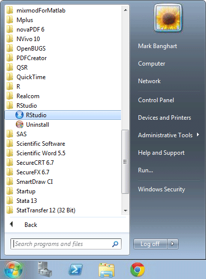
RStudio Start screen
RStudio window
RStudio's window looks like the following. Its Window is divided into panes. If no source files are open, the top left pane will not be displayed.
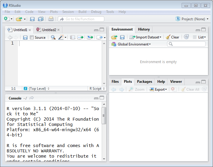
RStudio IDE screen
The size of the panes can be adjusted by moving the gray lines which separate the four panes. The panes can be minimized or maximized using the icons on the right side of the gray bar at the the top of each pane.
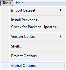
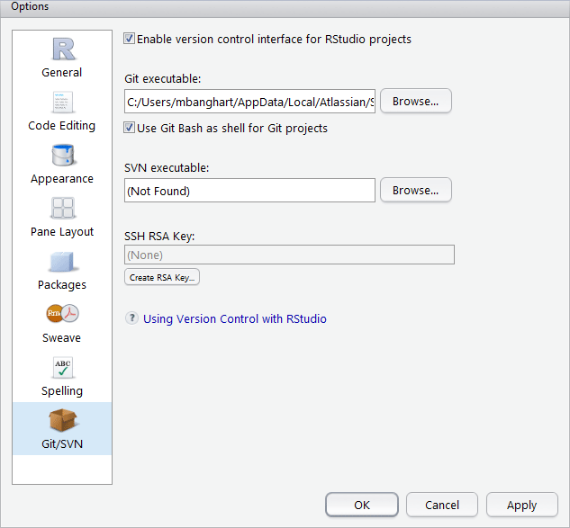
The location of the four panes within the window can be changed using the Pane Layout window. This window is accessed by selecting Global Options from the Tools drop down menu. The tool tabs can be moved between the two tab panes using this window as well. Navigation to the Pane Layout window is shown below
Console pane
The Console pane is on the left side on the bottom. This is where results are displayed. The console tab is opened when RStudio is opened. Additional tabs within this pane are opened if another program type is used, such as an R markdown file. This pane might be full height on the left side if no file is open in the source pane.
Source / Editor pane
The source pane is on the left side on top. This is where you will write and edit your R programs and documents. The pane will have a tab for each open file. This pane is only present if there are files opened in the editor.
The other panes; Environment, History, Git, Files, Packages, Plots, Help
There are two Tab panes on the right side, one on top and the other on the bottom. These panes contains tabs which allow quick access to additional tools. The tabs are for the following functions.
- Environment displays data objects defined in the current R session.
- History is a list of prior commands which have been executed.
- Git is used for version control.
- Files is a folder browser.
- Plots displays plots you create.
- Packages is where packages can be installed and loaded from.
- Help is where help on R commands can be found.
- Viewer is where web content can be viewed.
Console Basics
The basics of using the console are as follows.
- > is the command prompt. R will not display the command prompt until it has completed running the prior command. If the prompt is not displayed, R is not ready for a new command.
- + is the prompt for the continuation of a command. If R reaches the end of a line and the current R command is not complete, R assumes the next line continues the prior line. Splitting some commands across multiple lines can improve the readability of you source code by allowing the structure of the command or data to be seen visually.
- The escape key will end a command. This is handy if R thinks the current command is not finished and you see an error in what has already been entered.
- The page up and page down keys are used to scroll through the history of prior commands. A prior command can be recalled from the history, edited if needed, and then run again.
A few examples
Entering
3 * 5 + 1at the > prompt displays
[1] 16and the > prompt is displayed again.
Entering
3 * 5 +displays the + prompt. R knows that the command is not complete and is waiting for the rest of the command. Entering the following
1at the + prompt results in
[1] 16and the > prompt is displayed again.
Entering
(3 * 5 + 1)) / 2at the > prompt displays
Error: <text>:1:12: unexpected ')'
1: (3 * 5 + 1))
               ^
Note, your error messages maybe formated sightly differently, because the code in this document is run automatically.
Error messages result in a command being aborted. The > prompt is displayed after an error.
Typing code directly into the console is not reproducible. To make your research reproducible, R code should be written in a script file. The script file should be part of a project. We cover these topics next.
R Projects
A project in RStudio is a collection of work organized in a folder. RStudio provides tools that will help you manage your work on projects. Some of the many tools are,
RStudio remembers what files you had open and what tabs were displayed, when you close a project. When you open the project again, RStudio will open the same files and display the same tabs. This will allow you to quickly pick up your work again. A new R session is started when you open a project, so some previously executed commands may need to be run again.
Additional debugging tools, such as setting break points.
Integrated source control. This is an important part of reproducible code.
Integration of code results with documents.
Almost any R work can be structured as a project. You might consider creating a project for an individual class, your thesis, or a research project. While RStudio can work with individual files which are not in a project, you will likely find it quicker to develop R code using projects.
Creating a project
RStudio can create new projects using three different methods, New Directory, Existing Directory, or Version Control. All three of these method can be useful. For new users to R will likely want to use the New Directory method to get started. As your R knowledge and skills increase the other methods may be needed. To create a new project, select New Project from the file drop down menu.
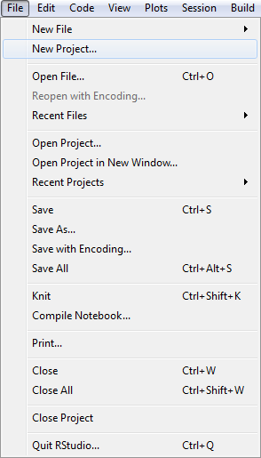
IDE Existing Project
The New Project window will allow you to select which method of project creation you want.
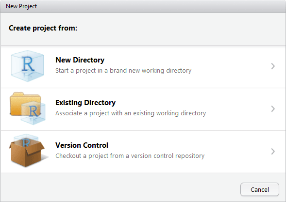
IDE New Project menu
The New Directory option is used when a new project is being started. This will create a .Rproj file and at the user's request start source control for the project.
You will have the option to create an Empty Project or an R Package. Packages are written by experienced R programmers. R Packages allow you to share finished R code with others users.
The Empty Project is what most new R users will use.
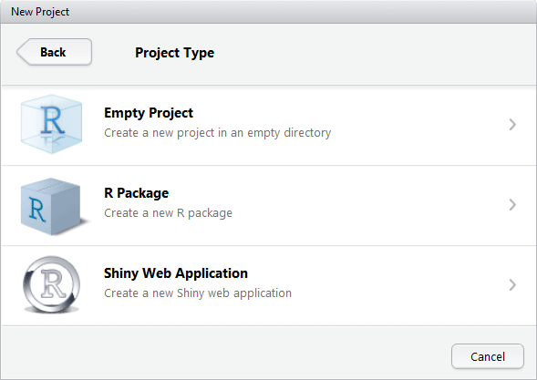
IDE New Project new directory
The Existing Directory option is used to create a project in a directory which already contains R programs. This will create the RStudio project (the .Rproj file), but does not set up source control for this project.
The Version Control option is used to start a local project folder from an existing project, provided the existing project is using Git. This is often a project which is shared by researchers.
Opening a project
An existing project can be opened by double clicking on the .Rproj file from a file browser. An existing project can also be opened within RStudio from either the Open Project or Open Project in New Session from the File dropdown menu, as displayed below.
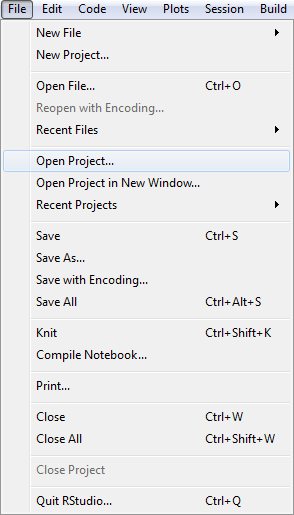
IDE Open Project
An Open Project window will be displayed. Navigate to the project folder. Select the file with extension .Rproj.
Scripts
An R script is a series of commands in a file. Scripts are ordinary text files with a file extension of .R. Commands can sent to the console from a script using the Run icon at the top of the Source pane.
A new script is created by selecting New File and then R Script from the File drop down menu.
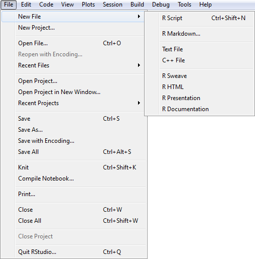
RStudio New File Menu
Scripts are edited in the Source pane. Remember to do regular saves when editing a script.
Commands / syntax
Functions
An R function is similar to a Stata and SAS command. A function performs some action and the action taken is adjusted based on the parameters given.
Syntax and use of functions
functionName(parameterList)
functionName is the name that identifies the function in R.
parameterList is a list of parameters. Parameters in the list are separated by commas. Parameters can be identified by either their position in the list or by a name. In most instances using the parameter name enhances the readability of your code. There is one case where dropping the use of parameter name is preferred, this is when the function name makes it clear what the first parameter is. This would look something like
parm1value, parmName = parmValue, ...
An R function returns an object as its result.
There are functions you will likely want to use which are in packages that will need to be explicitly loaded. This will typically be done in your scripts. Loading additional packages is covered at the end of this article.
A few examples
Entering
set.seed(7245052)returns no information to the console.
This call to set.seed() is an example of a parameter being identified by position. The value 7245052 will be used as the seed for future random numbers. Identifying 724052 with a parameter name as in set.seed(seed = 7245052) does not provide any additional information about how 724502 will be used by set.seed().
The set.seed() function is used when any random information will be generated.
Entering
help(set.seed)returns no information to the console. The help() function instead displays information in the Help tab. The Help tab now displays information on the set.seed() function. The help file for set.seed() shows that there are other parameters which can be used for set.seed().
This is another example of the first parameter being identified by position.
Entering
round(pi, digits = 2)displays the value of pi rounded to two significant digits.
[1] 3.14This is an example of using both positional and named parameters.
Entering
seq(from = 1, to = 50, by = 2)returns a sequence of numbers from 1 to 50 to the console.
 [1]  1  3  5  7  9 11 13 15 17 19 21 23 25 27 29 31 33 35 37 39 41 43 45
[24] 47 49
This example used 3 named parameters. One could have also used positional parameter identification and the parameters' default values to write seq(,50,2). While this would be far more concise, it would be difficult to read for all but highly experienced R programmers. A more middle ground approach to identifying the parameters would be seq(1, 50, by = 2). This would require the reader to know that 1 and 50 are the start and end values of the sequence while not requiring them to remember what the third parameter to seq() is.
Note, the [1] at the start of the first line indicates the element number displayed at the start of the row. Each row of the display will have an element number displayed. This is helpful when the display values are not a simple count.
Entering
c(3, 4, 9)combines 3, 4, and 9 into a vector of values and displays the vector.
[1] 3 4 9This is an example of a number of parameters being used with no parameter names.
The c() function is a special case of naming parameters in that names givn to these values are used as names in the vector. An example of this can be seen by entering the following.
c(one = 3, two = 4, three = 9)displays
  one   two three
    3     4     9
Commands
R commands are similar to commands from general computing languages like C++ or python. This is a little different from the syntax of languages such as Stata or SAS. R commands typically either assign values to an object or control which commands will get run.
Assignment command syntax and usage
object <- expression
Object is set to the value of expression.
<- is the assignment operator.
An Expression in R is any text which, when interpreted in R, results in a data object. Beneath this simple definition is one of the powerful constructs of R. An expression can also be used anywhere that a value is expected. This allows simple functions to be linked together to do much more sophisticated operations.
Expressions are numeric, logical, or character values with their associated operators. These values can be a variable, a constant, or the returned value from a function.
The numeric operators include +, -, *, /, ^, log(expression), exp(expression) which are addition, subtraction, multiply, divide, natural log, and the constant \(e\) raised to the power given by expression respectively.
The logical operators include: == the logical test for equality, < less than, <= less than or equal, > and >= similarly are greater, | logical or, & logical and.
Implied print command syntax and usage
expression
This is the same as the assignment command except instead of assigning the results of the expression to a data object, the results are displayed in the console.
A Comment is text to remind yourself, and others, of how to use your code and how it works. Comments are ignored (not treated as commands) by R.
# reminder text
- Comments start with a # and continue to the end of the current line. Comments can start at the first character of a line or may follow a command.
Conditional execution
The syntax and use of the if else command
if ( < logical expression > ) {
    < commands run if true >
} else {
    < commands run if false >
}
< logical expression > is any expression which can be coerced (i.e. turned into) to scaler logical value.
The else { } clause is optional and can be dropped if there are no commands needed for the FALSE condition of < logical expression >.
Looping
The syntax and use of the for command
for ( < object > in < values > ) {
    < commands >
}
The < commands > within the { } will be run once for each element of < vector >. < Object > will be assigned a value from < vector > each time the < commands > are run.
A few examples
Entering
student <- c("Maya", "Omar", "Emma", "Roy",
             "Aki", "Sara", "Jabari", "Tim")
assigns the eight names to the student object.
Entering
math <- round( runif(8, min = 10, max = 36), digits = 0)assigns eight values to math.
The right hand side demonstrates combining functions within a command. The random uniform, runif(), function returns 8 random values from the range 10 to 36. These 8 values are then passed into the round() function. The result is 8 random integers. These eight values can be displayed by entering the following.
math[1] 15 27 26 17 31 29 19 12Entering
if (format(Sys.time(), "%H") > 12) {
  timePeriod <- "PM"
} else {
  timePeriod <- "AM"
}
timePeriod
determines if the period of the day is AM or PM.
[1] "AM"The if condition is another example of combining functions within a command. The Sys.time(), function returns date and time information. The format() function returns just the hour portion of this information. The hour information is then compared to 12 in the if else command.
Entering
j <- 0
for (i in seq(1,5)) {
  j <- j + i
  print(c(i, j))
}
displays the first five triangular numbers.
[1] 1 1
[1] 2 3
[1] 3 6
[1]  4 10
[1]  5 15
Functional and object oriented constructs
R is a multi paradigm programing language supporting both functional programing and object oriented programing concepts. Most users will only use the functional programming paradigm. Users who move into writing packages and more advanced code will typically make use of R's object orient capabilities.
The most common place typical users will notice the object oriented programming of R is in the apparent overloading of function names. The summary() function is an example of this. The summary function will produce different results based on the nature of the first parameter. If a data set is the first parameter, summary() will summarize each variable in the data set. If the first parameter is a regression result, then a summary of the regression is provided. Behind the scenes in R, the summary function is calling different summary functions based on the first parameter, such as summary.data.frame() for a data set or summary.lm() for the results of a linear regression. This is called dispatching. The user does not need to remember which summary function to call. The user just calls summary() and R uses the right function for the object of interest.
Data
Data types and structures
Data objects have a type and can be organized in structures. A type is the form of what is being stored. Structures provide the relations between what is stored. This can be thought of as: a type defines which atom is used and the structure defines what elements, molecules, and compounds are built from atoms.
R is loosely typed. This means that R will coerce a variable to the type needed, if it can. What R does for a coerced variable is create a new variable with the needed type and passes this new variable to the function or expression. The original variable's type is not changed. So object types in R are a little less restrictive than in some other languages.
Some of the common data types are,
- Numeric which is a collection of types. R internally uses Integer, double, num, etc. for numeric variables. You will typically not need to be concerned about integer versus double, etc., since R will coerce where needed.
- Character is a string of characters.
- Logical variables take the value of either TRUE or FALSE, abbreviated as T and F. Numeric values coerced to logical assign FALSE for 0 and TRUE for all other values.
- Factor variables are stored as integer values. Depending where it is used, a factor may be used as either a numeric, character, or a set of indicator variables.
Some of the common structures are,
A vector is a one dimensional structure of elements. The elements of the vector must be of the same type. A vector is a single column and the elements of the vector are the rows of the column. Vectors can be of any length.
A data.frame is a two dimensional structure, even if there is only a single column in the data.frame. The columns of the data.frame are vectors. The vectors need to be the same length. The vectors do not need to be of the same type and often are not. It is common for a data set to be organized such that the vectors are the variables and each row is an observation.
A data.frame is the equivalent of Stata's data set.
A list is a one dimensional structure of elements which can contain elements of different types.
A matrix is a two dimensional structure with each column having the same type.
There are no scalar structure in R. A single value is a vector of length one.
A few examples
Entering
str(math)displays math's type as numeric and its structure is a vector (single dimension.)
num [1:8] 15 27 26 17 31 29 19 12Entering
act <- data.frame(student,
                  math,
                  english = round( runif(8, min = 10, max = 36), digits = 0)
                 )
creates a data.frame which includes the vectors student, math, and english.
Matrices and lists are created similarly using the matrix() and list() function. The c() function is typically used for creating vectors.
Entering
str(act)displays act's structure as a data.frame which contains 3 variables of 8 observations.
'data.frame':   8 obs. of  3 variables:
 $ student: Factor w/ 8 levels "Aki","Emma","Jabari",..: 4 5 2 6 1 7 3 8
 $ math   : num  15 27 26 17 31 29 19 12
 $ english: num  22 17 21 20 15 10 11 31
Entering
is.numeric(student)displays FALSE since student's type is character.
[1] FALSEThere is an similar is. type function for all core types (non user defined.)
Entering
as.logical(math)forces all the elements of math to be logical and displays all the elements. The elements are all TRUE, since math contained no elements with the value zero.
[1] TRUE TRUE TRUE TRUE TRUE TRUE TRUE TRUEThere is an similar as. type function for all core types (non user defined.)
Importing and exporting data sets
The act data.frame is an example of an R data set. This data set can be saved to a file using the write.table() function.
As an example we will save the act data.frame as a .csv file (comma separated values.)
write.table(act, file = "act.csv", sep = ",", row.names = FALSE)
R allows multiple datasets to be loaded in memory simultaneously. Each dataset is given a name when it is loaded or created to distinguish it from other datasets.
The most common way data is loaded to R is through .txt and .csv files. The data in these files will be organized with each line of the file representing one observation. The variables associated with each observation are separated in the rows by a special character such as a comma, blank space, tab, etc. These files are input into R using the read.table() function.
Syntax and parameters for the read.table() function
name <- read.table("filePath",parameters).
A data.frame is returned.
Name is the name you are giving the dataset in R.
FilePath is the path and name of the data file on your computer. If the file is in the work directory, then only the file name, with the file extension, is needed. If the file is in another folder, the path to the folder needs to be provided with the file name.
In R the backslash, \, is the escape character. To use this in the filePath, you would use, \\. On a Windows machine, one can also use the forward slash, /, in place of the backslash, since windows will accept both from R. Either, "u:\\projects\\datafile.csv" or "u:/projects/datafile.csv" would be accepted as a filePath.
Some commonly used parameters are
header set to FALSE indicates no column names are present. TRUE indicates column names are in the first row. Header has no default value. If header is not present in the function call, the presence of a header row is determined from the first row of the data file. If the first row has one less value than the rest of the data, the first row is assumed to be column names.
sep is a character string and defaults to "", the empty character. "" indicates that any white space is used as a separator.
As an example we will load the act.csv file.
act <- read.table("act.csv", sep = ",", header = TRUE)The act data.frame that we created with the data.frame() function was overwritten by the assignment from the read.table() function.
Subseting structures
R allows you to use all or just some of the elements of a structure. There are several methods for referencing some of elements of a structure. One method to subset a structure is to use [row,column] indexing. Another method, when a column is named, is to use object$columnName indexing.
A few examples
Entering
act[c(2,6),]displays all variables for observations 2 and 6.
  student math english
2    Omar   27      17
6    Sara   29      10
This subseting results in a data.frame of three variables with two observations.
If the rows of the data.frame had non-numeric names, those names could be used to subset on as well.
Entering
act[,c("student", "english")]displays all observations for variables student and english.
  student english
1    Maya      22
2    Omar      17
3    Emma      21
4     Roy      20
5     Aki      15
6    Sara      10
7  Jabari      11
8     Tim      31
This subseting results in a data.frame of two variables with eight observations.
Entering
act$english[4:7]dispalys the values of the english variable in observations 4, 5, 6, and 7.
[1] 20 15 10 11There are two different subsetting operations in this example. A single variable, english, is selected from the act data.frame using act$english. This is now a vector. So this single dimensional. The rows of act$english vector are subsetted by 4:7, which is a another way of stating seq(4,7, by = 1).
Entering
act$student[act$english > 30]displays names of all students who scored greater than 30 on the english portion of our imaginary act test.
[1] Tim
Levels: Aki Emma Jabari Maya Omar Roy Sara Tim
In this example the subsetting was done using a conditional test.
Referencing variables
The student variable was created as a vector. A copy of that vector was put in the act data.frame. They are two different vectors. Currently they have the same values. This can be seen by entering the following.
student## [1] "Maya" "Omar" "Emma" "Roy" "Aki" "Sara" "Jabari" "Tim"act$student## [1] Maya Omar Emma Roy Aki Sara Jabari Tim
## Levels: Aki Emma Jabari Maya Omar Roy Sara TimTo see that they are different vectors, enter the following.
student[1] <- "Chancy"
student
## [1] "Chancy" "Omar" "Emma" "Roy" "Aki" "Sara" "Jabari" "Tim"act$student## [1] Maya Omar Emma Roy Aki Sara Jabari Tim
## Levels: Aki Emma Jabari Maya Omar Roy Sara TimThe new name for student 1 is made to the student vector. The act$student vector is unchanged.
The english vector was created as a column of the act data.frame. There is no english vector separate from the act data.frame. This can be seen by entering the following.
english## Error in eval(expr, envir, enclos): object 'english' not foundA Few other useful functions for working with data
aggregate
The aggregate() function is used when you want to apply a function across groups of observations.
Entering
act$class <- c("A", "A", "A", "A", "B", "B", "B", "B")
aggregate(act[,c("math", "english")],
          by = list(act$class),
          FUN = mean
          )
divides the eight students into two imaginary classes then averages the math and english scores within each of these class groups.
  Group.1  math english
1       A 21.25   20.00
2       B 22.75   16.75
ifelse
The ifelse() function is used to conditionally assign values to a row.
Entering
ifelse(act$math > act$english, "English", "Math")displays a vector identifying which subject the student was stronger in.
[1] "Math"    "English" "English" "Math"    "English" "English" "English"
[8] "Math"
cut
The cut() function is used to divide a continuous numeric vector into groups based on cut points.
Entering
cut(act$english,
    breaks = c(0, 20,30,37),
    labels = c("Low", "Middle", "High")
    )
displays a the observations which are lower than 20, higher than 30, and in the middle.
[1] Middle Low    Middle Low    Low    Low    Low    High
Levels: Low Middle High
which
The which() function is used to identify which elements fit a particular condition.
Entering
which(act$math > act$english)displays a vector of the observation numbers for the students which are scored higher in math.
[1] 2 3 5 6 7A vector of index values is one way to retain subsetting information for later use. As an example this could be used to list the names of the students who scored better in math.
mathIndx <- which(act$math > act$english)
act$student[mathIndx]
[1] Omar Emma Aki Sara Jabari Levels: Aki Emma Jabari Maya Omar Roy Sara Timcolnames and rownames
The colnames() and rownames() functions are used to access the names given to the columns and rows of an object.
Entering
colnames(act)displays names of the variables in the act data set.
[1] "student" "math" "english" "class"Entering
rownames(act) <- act$studentsets the row names of the act data.frame to the students names.
factor
The factor() function is used to force any other type of variable to type factor.
Entering
factor(ifelse(act$math >= act$english, "English", "Math"))displays the vector which identifies which subject the observation was stronger in as a factor
[1] Math    English English Math    English English English Math
Levels: English Math
Factor variables are stored as numeric values. Factor variables can then be converted to numeric and mathematical operations can then be done with them. For example
cor(as.numeric(factor(act$class)), act$english)determine the correlation between the english scores and the two classes
[1] -0.2569853
Packages
The packages which make up the core functions and commands of R are loaded when R is started. There are many packages which extend R's capabilities beyond the core. These extension packages need to be loaded in each R session before you can use the functions they contain. The functions in these extensions range from widely used functions to obscure functions used by only a small number of people.
A package needs to be installed on your computer before you can load it into your session. R and RStudio manage a library of packages that have been installed on your computer. Winstat has a number of common packages installed for you. The packages installed in your library can be seen in the packages tab.
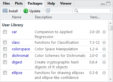
Packages tab
To install a package on your computer, click the Install icon in the Package tab and then enter the package you want installed.
library
The library() function is used to load a package into your R session.
library(packageName)
PackageName is the package which is to be loaded.
There is nothing displayed by this function.
Further reading
To learn more about using R and RStudio see R for Researchers.
Last Revised: 1/13/2017