R for researchers: Diagnostics
April 2015
This article is part of the R for Researchers series. For a list of topics covered by this series, see the Introduction article. If you're new to R we highly recommend reading the articles in order.
Overview
This article will introduce you to some of the functions commonly used to create model diagnostics. The article includes the use of the reshape() and merge() functions in preparing diagnostics. These two functions are also useful in preparing data sets.
Model diagnostics are typically done as models are being constructed. Model construction and diagnostics were separated into separate articles to provide a focus on the each of these important areas of modelling data. We recommend doing model diagnostics as models are being constructed.
Preliminaries
You will get the most from this article if you follow along with the examples in RStudio. Working the exercise will further enhance your skills with the material. The following steps will prepare your RStudio session to run this article's examples.
- Start RStudio and open your RFR project.
- Confirm that RFR (the name of your project) is displayed in the upper left corner of the RStudio window.
- Open your SalAnalysis script.
- Run all the commands in SalAnalysis script.
Review of Model from Regression OLS article
We will start our diagnostics using the model that we fit in the Regression (OLS) article. This model was saved as the outSin3 model object. All of the model terms, other than sex, are significant using the criteria of a nested F-test. The coefficients of the outSin3 model are shown below.
                 Estimate  Std. Error   t value     Pr(>|t|)
(Intercept)   60.37876235 5.329187300 11.329826 6.450180e-26
dscplB        14.19990425 2.331060758  6.091606 2.682402e-09
sexMale        5.23359783 3.860948265  1.355521 1.760360e-01
rankAssocProf  5.55108100 5.033353169  1.102859 2.707683e-01
rankProf      34.10087790 6.184018504  5.514356 6.382629e-08
yrSin          1.51262460 0.565502985  2.674830 7.791372e-03
yrSinSqr      -0.02503732 0.009508336 -2.633196 8.794875e-03
Model form diagnostics
An OLS model is assumed to be linear with respect to the predicted value with constant variance. This is typically checked visually with a plot of the residuals to the fitted values. The model form is accepted as correct if there are no observable change in the variance of the residuals (constant variance) and there is no pattern to the residuals (linear with respect to the predicted values.) The plot() function provides a residual plot for the model.
Syntax and use of the plot() function for model objects.
plot(modObj, which=plotId)
There is no returned object. Diagnostics plots are generated by this function.
plotId can take values from 1 through 6. The three plots we will examine are, 1 for a residual plot, 2 for the normal q-q of residuals, and 5 for the residual versus leverage plots. The default for plotId is c(1,2,3,5). When there are multiple plots produced from one call to plot, you will be prompted in the console pane to hit enter for each of these plots. This is to allow you time to view and possibly save each plot before the next plot is displayed.
This set of prepared diagnostic plots provides an initial look at all the major model assumptions and is a good place to start the evaluation of the fit of a model.
The following code produces the residual plot.
Enter the following command in your script and run it.
plot(outSin3, which=1)There are no console results from this command. The following plot is produced.
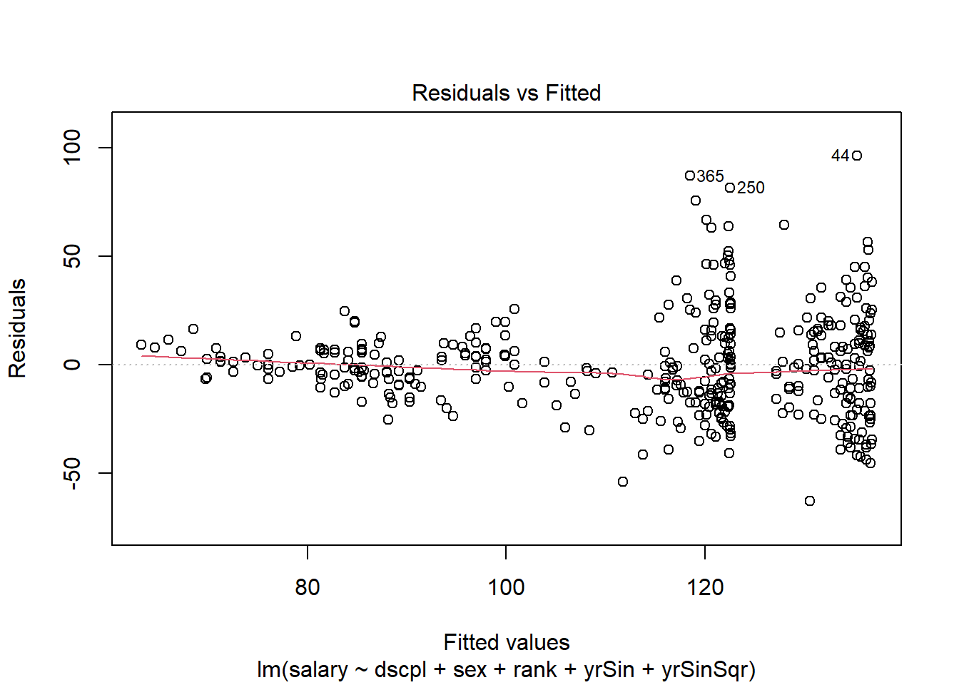
The residual plot shows increasing residual variance with increases in predicted salary. This is a concern with the form of our model.
Correcting the model form
What we have learned from this first diagnostic check is that the model we built in the last article is not appropriate. We will need to correct the model form.
There are many ways to correct the form of a model. We will correct the issues with the inconsistent variance using a weighted fit. We will use the assumption that there is a known variance for each rank and discipline groups. While this does not appear to fully explain the inconsistency in variance in our current model, the majority of the variance differences can be attributed to the group. We will estimate the known variance without accounting for this in our results. This short-cut of not correcting for the estimates of group variance and the simplifying assumption of the group variance being known are used in this article to allow the article to focus on the diagnostics. As with all models, the user is expected to understand the statistical theory for the model and use the model appropriately.
The variance of the groups are calculated using the aggregate() function. The data.frame returned from aggregate() has a row for each group and we need a value for each observation in salary. The merge() function can be used to add a variable to a data.frame when the new data does not have the same number of row as the data set.
Syntax and use of the merge() function.
merge(data1,data2,by=col)
Returns a data.frame.
This function merges data1 and data2 into one data.frame.
col is the columns to use for the merge. The default is to use all columns in data1 and data2 which have the same name.
The following code calculates the group variances and merges the variance variable with the salary data.frame. The weight variable is then added and the model is then fit with weights.
Enter the following command in your script and run it.
wGrp <- aggregate(list(var=salary$salary),
          by=list(rank=salary$rank,dscpl=salary$dscpl),
          FUN=var
          )        # find variance of groups

salWeight <- merge(salary,wGrp)   # add var to data set
salWeight$wght <- (1/salWeight$var) /  mean((1/salWeight$var))

salMod <- lm(salary~dscpl + sex + rank + yrSin + yrSinSqr,
             weights=wght,
             data=salWeight
             )
summary(salMod)$coefficients
The results of the above commands are shown below.
                  Estimate  Std. Error    t value      Pr(>|t|)
(Intercept)   70.851719534 2.128797183 33.2825128 5.242589e-116
dscplB        12.207552540 1.232182099  9.9072633  8.693466e-21
sexMale        2.135076469 1.611549370  1.3248595  1.859935e-01
rankAssocProf 13.386841228 2.194176989  6.1010763  2.541256e-09
rankProf      47.835983162 3.339265328 14.3253017  1.075425e-37
yrSin          0.161353128 0.290856911  0.5547509  5.793831e-01
yrSinSqr      -0.005143292 0.005478514 -0.9388115  3.484086e-01
The significance of yrSinSqr has been reduced to a level which would not be significant. Although the model could be reduced further, we will preliminarily accept this model to focus on the diagnostics in this article.
The residual plot generated by plot() uses the residuals on the scale of the variable. To check the fit of salMod we need to examine the residuals on the weighted scale. We will need to use an extractor function to obtain the weighted residuals.
Extractor functions
R has a number of extractor functions for model objects. Using extractor functions is a good programming practice, as opposed to directly getting the values from an object. If the underlying object is ever changed, your code will not need to be changed if you are using the extractor functions.
We will use a number of these extractor functions to obtain information about the model fit.
Syntax and use of model object extractor functions
Most of these extractors return a vector with an element for each observation which was used in the model fit. The model fit may have fewer observations than the data if there are observations with missing values or other problems with result in an observation failing to be included.
fitted(modelObj)
Returns a vector of the predicted y values.
residuals(modelObj)
rstandard(modelObj)
rstudent(modelObj)
weighted.residuals(modelObj)Returns a vector of the residuals, standardized residuals, studentized residuals, or the residuals on the weighted scale respectively.
hatvalues(modelObj)
Returns as a vector the diagonal of the projection matrix (hat matrix.) This is a measure of leverage.
cooks.distance(modelObj)
Returns a vector of the Cook's distance. This is a measure of influence.
vcov(modelObj)
Returns the variance covariance matrix for the coefficients.
The diagonals of this matrix are the square of the standard error reported in the the model summary.
We will create a new data.frame containing the variables used in the model and some diagnostic variables. We will name this data.frame salModDiag.
Enter the following commands in your script and run them.
salModDiag <- salWeight[,c("rank","dscpl","yrSin","yrSinSqr","sex","salary","wght")]
salModDiag$fit <- fitted(salMod)
salModDiag$res <- weighted.residuals(salMod)
salModDiag$cooks <- cooks.distance(salMod)
salModDiag$lev <- hatvalues(salMod)
There are no console results from these commands.
Plotting weighted residuals
We will now create a residual plot using the weighted residuals.
Enter the following command in your script and run it.
ggplot(salModDiag, aes(x=fit,y=res) ) +
  geom_point() +
  theme_bw()
There are no console results from these commands. The following plot is produced.
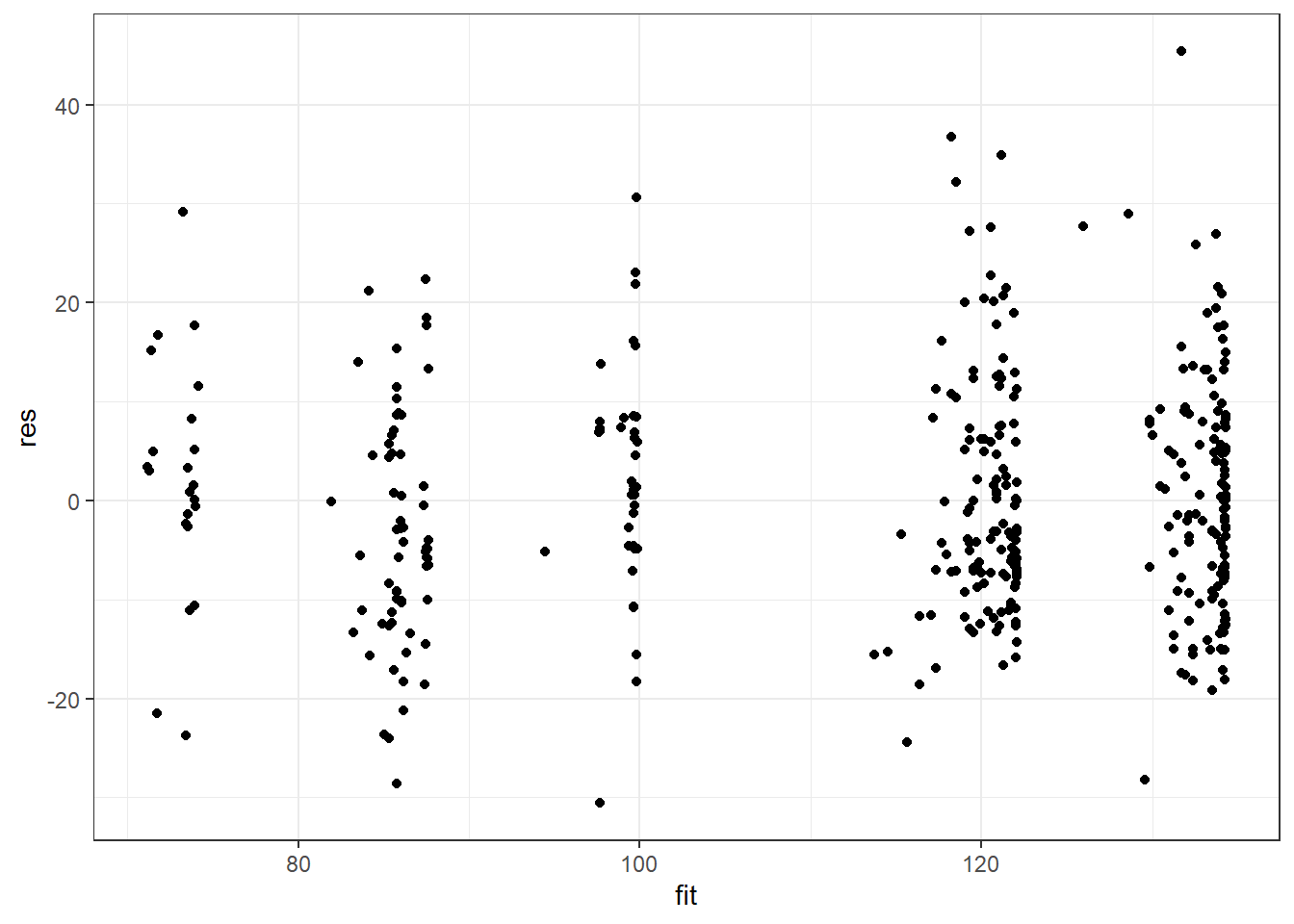
The model exhibits a much more consistent variance. There are no serious issues with model from with this weighted fit. We will continue our diagnostics using salMod.
Linearity in each variable diagnostics
It is also important to check for patterns in the plots of the residuals versus each of the variables of the model. We will use ggplot's faceting feature to make a residual plot for each of the variables.
Reshaping a data.frame to long form
The variables we would like to facet on are columns of the salModDiag data.frame. These columns are shown below. The many rows of data between 1 and \(n\) are represented with a single row of ".".
| res | rank | dscpl | yrSin | yrSinSqr | sex |
|---|---|---|---|---|---|
| \(r_1\) | rank\(_1\) | dscpl\(_1\) | ysSin\(_1\) | ysSinSqr\(_1\) | sex\(_1\) |
| . | . | . | . | . | . |
| \(r_n\) | rank\(_n\) | dscpl\(_n\) | ysSin\(_n\) | ysSinSqr\(_n\) | sex\(_n\) |
The salModDiag data.frame is in wide form with multiple model variables in a row with each observed residual value. We will need salModDiag in long form, also sometimes called tall form, with a separate row for each variable-observation pairing in the data.frame. This can be thought of as stacking each column of the variables into a single new column. In addition to this new column variable, we need a variable to identify which variable the long (stacked) observation belongs to. Long form would look like below.
| res | var | id |
|---|---|---|
| \(r_1\) | rank\(_1\) | "rank" |
| . | . | . |
| \(r_n\) | rank\(_n\) | "rank" |
| \(r_1\) | dscpl\(_1\) | "dscpl" |
| . | . | . |
| \(r_n\) | dscpl\(_n\) | "dscpl" |
| \(r_1\) | yrSin\(_1\) | "ysSin" |
| . | . | . |
| . | . | . |
| . | . | . |
| \(r_n\) | sex\(_n\) | "sex" |
Long form maintains the residual-variable pairing for each observation in the regression. That is in the long form there is row for the first residual paired with the rank of that model observation, a row for the first residual paired with dscpl of that model observation, and this is repeated for all the variables and all the observations in the model. There is no loss of information when converting between the two forms.
The reshape function is useful to change between wide (what we have) and long (what we want) or from long to wide form. We are going from wide to long so our use of reshape is
Syntax and use of the reshape() function.
reshape(df,varying=wide,v.names=rep,
\(\qquad\) timevar=id,times=lev,
\(\qquad\) drop=excld,
\(\qquad\) direction=dirct
\(\qquad\) )Returns a data.frame.
wide is character vector containing the names of the repeated variables in wide form. These are the variables which will be stacked in the long form.
rep is the name of the combined variable in the long data.frame.
id is the name of the identifier variable for the combined variable.
excld is a character vector of the names of variables in the data.frame which are to be excluded from the reshaped data.frame.
dirct is either "long" or "wide" and indicates which form to reshape to.
To create the single variable for the val column shown above, we need all the variables to be of the same type. As done in the Data exploration article we will changing the type of all the variables to numeric.
Enter the following command in your script and run it.
salModDiagNum <- salModDiag
for(i in colnames(salModDiagNum)) {
  salModDiagNum[,i] <- as.numeric(salModDiagNum[,i])
  }
There are no console results from these commands.
## Warning: NAs introduced by coercion

## Warning: NAs introduced by coercion
We will reshape using res, lev, and cooks as varying variables. We are including lev and cooks since we will plot these later in the article. This will create a column in long form for each of these three variables. The following code reshapes salModDiag to long form.
Enter the following commands in your script and run them.
salModDiagTall <- reshape(salModDiagNum,
                 varying=c("rank","dscpl","sex","yrSin","yrSinSqr"),
                 v.names="varVal",
                 timevar="variable",
                 times=c("rank","dscpl","sex","yrSin","yrSinSqr"),
                 drop=c("salary","fit"),
                 direction="long"
                 )
str(salModDiagTall)
The following is the console results from these commands.
'data.frame':   1985 obs. of  7 variables:
 $ wght    : num  1.14 1.14 1.14 1.14 1.14 ...
 $ res     : num  -4.87 -14.5 -11.34 -8.36 17.69 ...
 $ cooks   : num  0.000547 0.005427 0.004593 0.00276 0.007552 ...
 $ lev     : num  0.0216 0.0241 0.0328 0.036 0.0226 ...
 $ variable: chr  "rank" "rank" "rank" "rank" ...
 $ varVal  : num  2 2 2 2 2 2 2 2 2 2 ...
 $ id      : int  1 2 3 4 5 6 7 8 9 10 ...
 - attr(*, "reshapeLong")=List of 4
  ..$ varying:List of 1
  .. ..$ varVal: chr [1:5] "rank" "dscpl" "sex" "yrSin" ...
  .. ..- attr(*, "v.names")= chr "varVal"
  .. ..- attr(*, "times")= chr [1:5] "rank" "dscpl" "sex" "yrSin" ...
  ..$ v.names: chr "varVal"
  ..$ idvar  : chr "id"
  ..$ timevar: chr "variable"
Plotting residuals versus each variable
We can now plot the residuals against each of the model variables.
Enter the following command in your script and run it.
ggplot(salModDiagTall, aes(x=varVal, y=res) ) +
  geom_point() +
  facet_wrap(~variable, scales="free_x") +
  theme_bw() +
  theme(strip.background = element_rect(fill = "White"))
There are no console results from these commands. The following plot is produced.
## Warning: Removed 794 rows containing missing values (geom_point).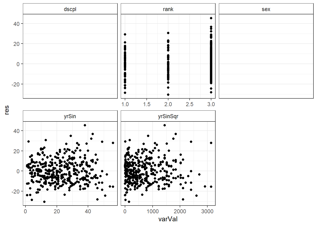
There is no significant indication of non-linearity in any of the variables. While there is some slight indication of inconsistent variance with respect to yrSin, we will continue to use our model based on the simplifying assumption made above.
Independence
The independence of observations assumption has limited diagnostics. This assumption is mainly examined by considering the randomization used in the study design. A check for autocorrelation is sometimes done. We will not cover autocorrelation tools in this series.
Normality of residuals diagnostics
Normality of the residuals is typically checked with with a q-q plot (quantile-quantile.) Linearity of the observations and symmetric scales indicate little concern for deviations from normality.
A q-q plot of the residuals is produced by the plot() function.
Enter the following command in your script and run it.
plot(salMod,2)There are no console results from this command. The following plot is produced.
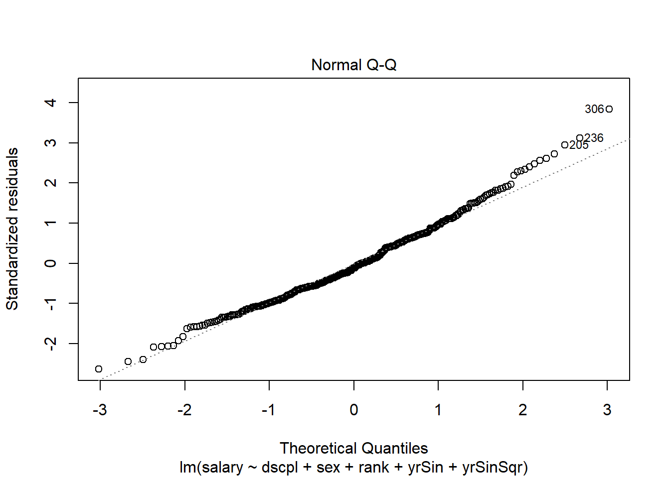
The above plot uses the residuals from the original scale. We need to examine the weighted residuals (the scale that was used in the fit.) We will do this using the qqnorm() function.
Syntax and use of the qqnorm() function.
qqnorm(vec)
There are no returned results for this function. A plot is generated from the function.
vec is the vector of values to be compared to normality.
The code for our weighted residuals is shown below.
Enter the following command in your script and run it.
qqnorm(salModDiag$res)There are no console results from this command. The following plot is produced.
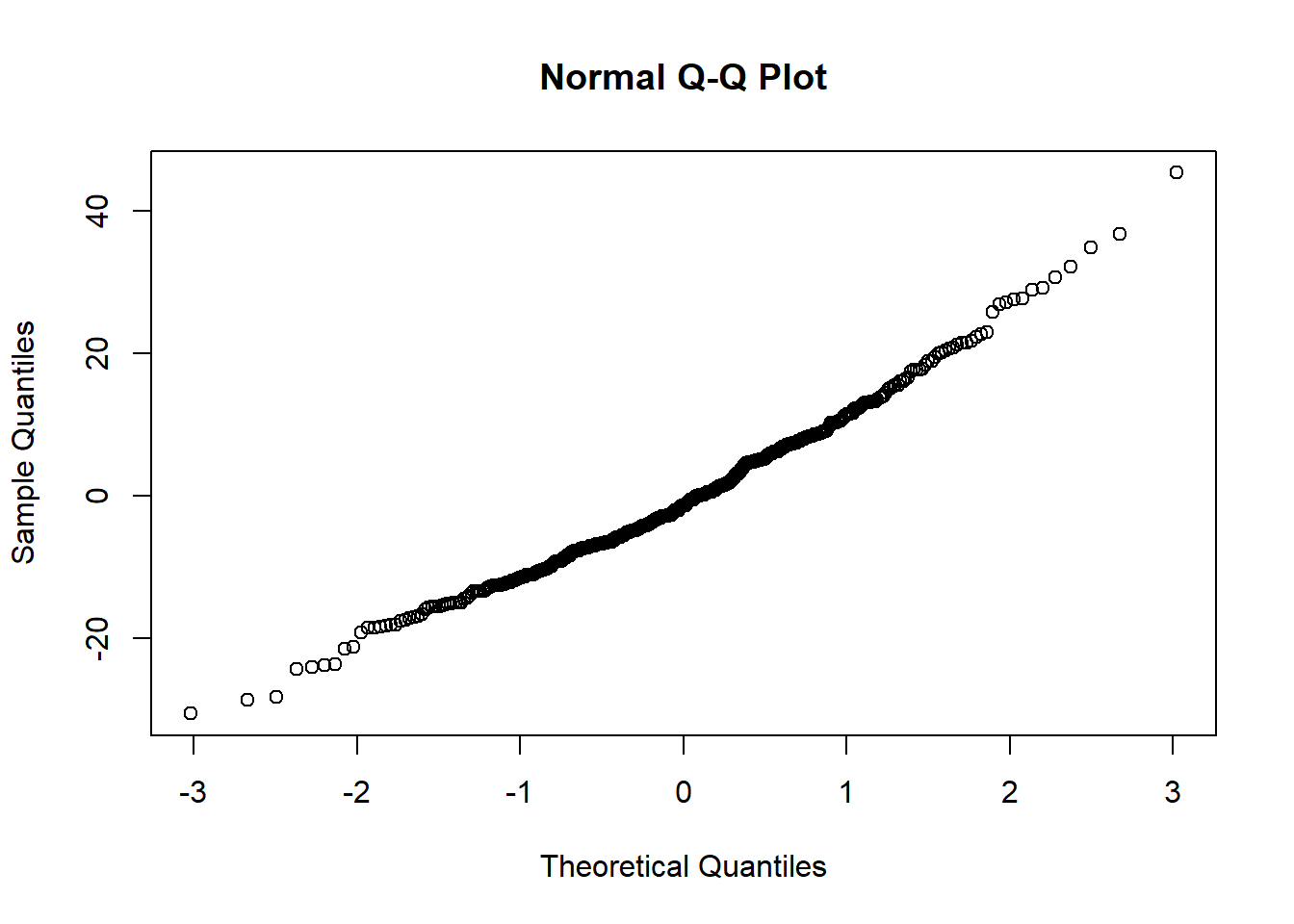
The quantile plot (also called a normal probability plot) does not raise any significant concern with normality of the weighted residuals.
Sensitivity to data diagnostics
It is important to check that your model is not influenced by one or a small set of observations. This might indicate your model is over fit.
The residuals vs. leverage plot from the model object plot provides a good view of the sensitivity of the model to a single or a small set of observations. The leverage of the observations is plotted on the x-axis. The leverage measure used is the diagonal of the hat matrix and is a measure of the distance of the observation from the mean observation of the set. The cooks distance for the observations are given in interval bands in the plot.
The residual vs. leverage plot for our model is generate with the plot() function.
Enter the following command in your script and run it.
plot(salMod,5)There are no console results from this command. The following plot is produced.
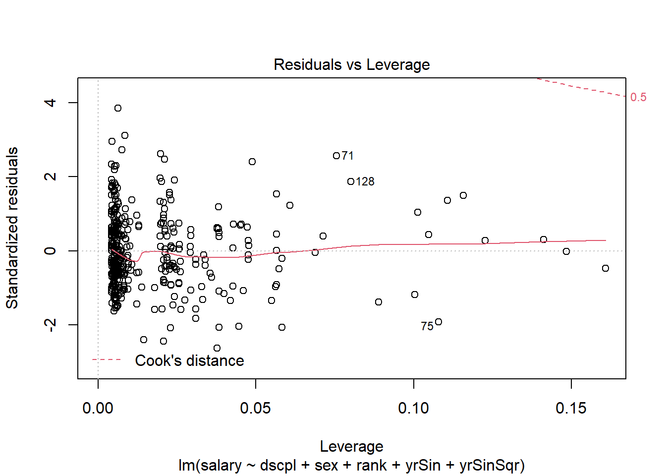
The residuals in this plot are the standardized residuals from the scale of the variable. This is not the weighted scale that is of interest. This does not detract from our ability to use the leverage and Cook's distance from the plot.
In our plot you can see in the upper right corner the band for a cooks distance of 0.5. There are no observations close to this band; the Cook's distances are generally small. There is no indication that any single observation is exerting influence. There are several observations with slightly higher leverage values than the rest of the observations. The investigation of these observations follows.
Examining leverage and influence observations
The plots of leverage and influence to each of the model variables can be useful to visually examine if there is a cluster of observations influencing the fit.
We have leverage and Cooks distance in long form in the salModDiagTall data.frame. So, we can plot these diagnostics faceted by the model variables.
Enter the following commands in your script and run them.
ggplot(salModDiagTall, aes(x=varVal, y=lev) ) +
  geom_point() +
  facet_wrap(~variable, scales="free_x") +
  theme_bw() +
  theme(strip.background = element_rect(fill = "White"))
ggplot(salModDiagTall, aes(x=varVal, y=cooks) ) + geom_point() + facet_wrap(~variable, scales="free_x") + theme_bw() + theme(strip.background = element_rect(fill = "White"))There are no console results from this command. The following plots are produced.
## Warning: Removed 794 rows containing missing values (geom_point).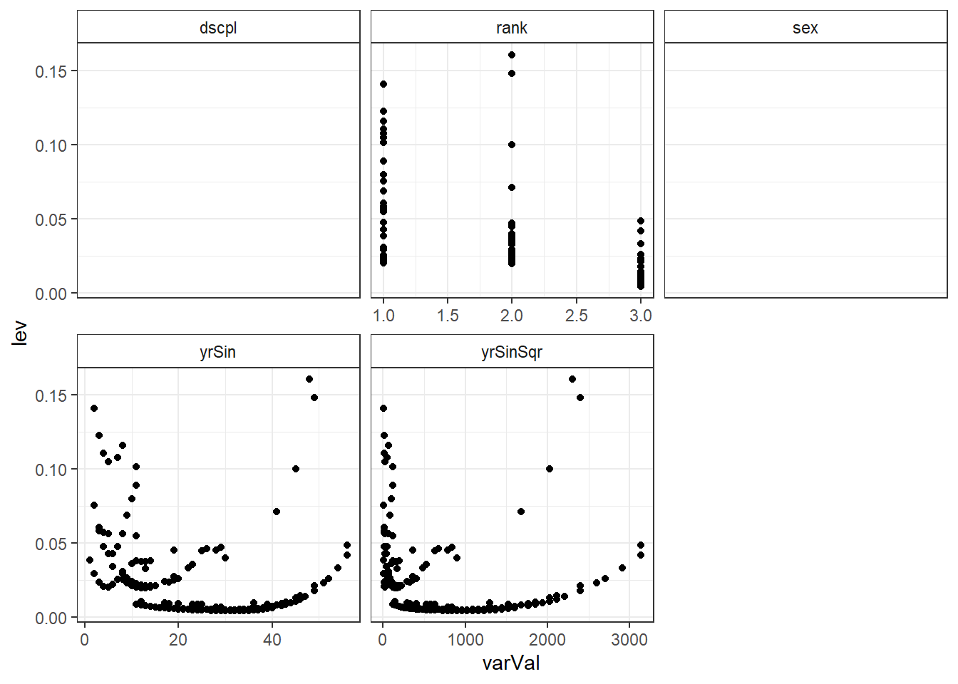
## Warning: Removed 794 rows containing missing values (geom_point).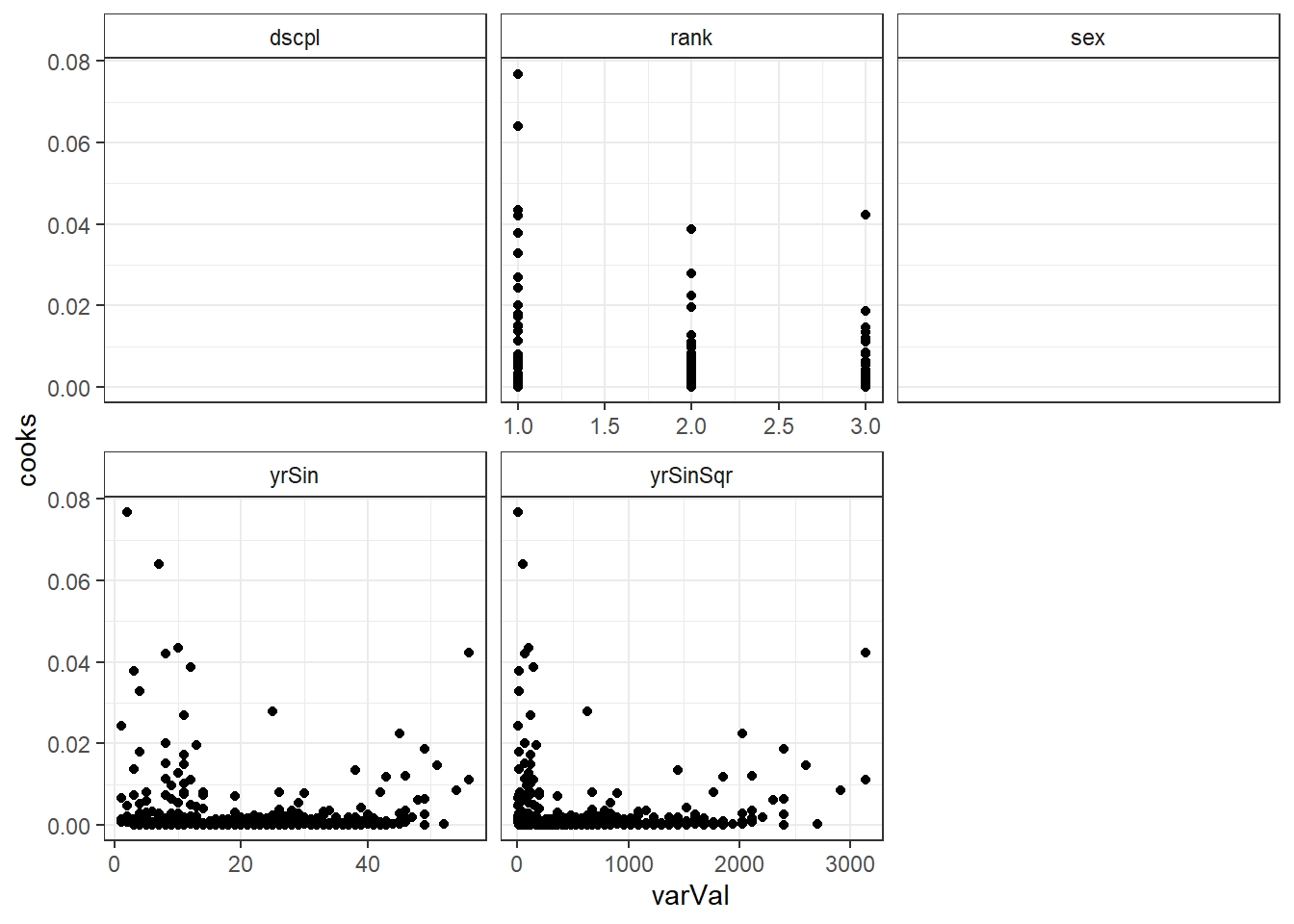
There are two observations with higher leverage values that have the same rank and sex. There is also two observations with a slightly higher Cook's distance, though not high enough to individually be of concern.
Excluding observations to examine sensitivity of the model
It is important to investigate the sensitivity of a model to an observation or set of observations with either higher influence, higher leverage, or residual outliers. There were no residual outliers on the weighted scale in our model. We will examine the sensitivity of the model to the cluster of observations seen in the leverage and Cook's distance plots above.
To know if an observation, or set of observations, is impacting the fit of a model, the observations can be removed and the model refit. The difference between the two models can be examined to determine if any change is of concern. Removing the observation is solely for the purpose of evaluating the sensitivity of the fit to the data. It is not recommended to remove observations from a model to improve the fit.
We will remove the three observations which had leverage values higher than .145. We will use the which() function to identify these observations.
Enter the following commands in your script and run them.
salModLevId <- which(salModDiag$lev >= .145)
salModDiag[salModLevId,c("salary","rank","dscpl","sex","yrSin")]
The results of the above commands are shown below.
   salary      rank dscpl  sex yrSin
8    81.8 AssocProf     A Male    49
44   90.0 AssocProf     B Male    48
We can now run the same model with these three observations removed.
Enter the following commands in your script and run them.
salModLev <- lm(salary~dscpl + sex + rank + yrSin + yrSinSqr,
                weights=wght,
                data=salModDiag[-salModLevId,])
summary(salModLev)
The results of the above commands are shown below.
Call:
lm(formula = salary ~ dscpl + sex + rank + yrSin + yrSinSqr,
    data = salModDiag[-salModLevId, ], weights = wght)

Weighted Residuals:
    Min      1Q  Median      3Q     Max
-30.640  -7.931  -1.326   7.448  45.265

Coefficients:
               Estimate Std. Error t value Pr(>|t|)
(Intercept)   70.870042   2.136867  33.165  < 2e-16 ***
dscplB        12.254717   1.239995   9.883  < 2e-16 ***
sexMale        2.135023   1.615298   1.322    0.187
rankAssocProf 13.412374   2.202293   6.090 2.72e-09 ***
rankProf      47.530649   3.428175  13.865  < 2e-16 ***
yrSin          0.149705   0.293727   0.510    0.611
yrSinSqr      -0.004484   0.005777  -0.776    0.438
---
Signif. codes:  0 '***' 0.001 '**' 0.01 '*' 0.05 '.' 0.1 ' ' 1

Residual standard error: 11.87 on 388 degrees of freedom
Multiple R-squared:  0.6895,    Adjusted R-squared:  0.6847
F-statistic: 143.6 on 6 and 388 DF,  p-value: < 2.2e-16
Since both models were run with the same variables in the same order, we can directly compare the vectors of coefficients. We will calculate the difference in the coefficients between the two models. Then scale this difference using the standard error from the model with all the observations to standardize the differences.
Enter the following commands in your script and run them.
salModLevCD <- data.frame(change=(coef(salModLev) - coef(salMod)),
                         se=sqrt(diag(vcov(salMod)))
                         )
rownames(salModLevCD) <- names(coef(salMod))
salModLevCD$multiples <- salModLevCD$change / salModLevCD$se
salModLevCD
The results of the above commands are shown below.
                     change          se     multiples
(Intercept)    1.832236e-02 2.128797183  8.606906e-03
dscplB         4.716442e-02 1.232182099  3.827715e-02
sexMale       -5.378637e-05 1.611549370 -3.337556e-05
rankAssocProf  2.553279e-02 2.194176989  1.163661e-02
rankProf      -3.053338e-01 3.339265328 -9.143741e-02
yrSin         -1.164779e-02 0.290856911 -4.004644e-02
yrSinSqr       6.595420e-04 0.005478514  1.203870e-01
The changes in all the coefficients are within the confidence intervals for the coefficients. These changes are not large enough to cause a concern about the model being sensitivity to these observations. There is no indication that the model is being overly influenced by these observations.
We will repeat the same examination of the two higher Cook's distance observations.
Enter the following commands in your script and run them.
salModCooksId <- which(salModDiag$cooks >= .06)
salModDiag[salModCooksId,c("salary","rank","dscpl","sex","yrSin")]

salModCooks <- lm(salary~dscpl + sex + rank + yrSin + yrSinSqr,
                weights=wght,
                data=salModDiag[-salModCooksId,])

salModCooksCD <- data.frame(change=(coef(salModCooks) - coef(salMod)),
                         se=sqrt(diag(vcov(salMod)))
                         )
rownames(salModCooksCD) <- names(coef(salMod))
salModCooksCD$multiples <- salModCooksCD$change / salModCooksCD$se
salModCooksCD
The results of the above commands are shown below.
   salary     rank dscpl    sex yrSin
71   85.0 AsstProf     A   Male     2
75   63.1 AsstProf     A Female     7
change se multiples (Intercept) -0.108445154 2.128797183 -0.05094199 dscplB 0.303529370 1.232182099 0.24633483 sexMale -1.155809111 1.611549370 -0.71720366 rankAssocProf -0.874136926 2.194176989 -0.39838943 rankProf -1.339983427 3.339265328 -0.40128091 yrSin 0.178159890 0.290856911 0.61253449 yrSinSqr -0.002970411 0.005478514 -0.54219275
There is no indication that the model is overly influenced by these two observations with higher Cook's distance.
If there were residual outliers, their effect on the model would be checked using the same approach.
Multicollinearity
The vif() function will return the variance inflation factor for the model variables. There are two versions of vif() in the packages we have loaded. We are using the version from the cars package; it has overwritten the version from the faraway package.
Syntax and use of the vif() function.
vif(modelObj)
Returns a matrix with a row for each model term.
Enter the following command in your script and run it.
vif(salMod)The results of the above command are shown below
              GVIF Df GVIF^(1/(2*Df))
dscpl     1.074880  1        1.036764
sex       1.030136  1        1.014956
rank      4.233630  2        1.434426
yrSin    23.514956  1        4.849222
yrSinSqr 15.442166  1        3.929652
The vif scores are elevated for the two variables based on yrSin. We would expect these two variables to have higher vif scores since the variables are correlated. If vif is a concern, it would be more informative to check vif on the model which uses poly() for higher order terms.
Exercises
These exercises use the alfalfa dataset and the work you started on the alfAnalysis script. Open the script and run all the commands in the script to prepare your session for these problems.
Note, we will use the shade and irrig variable as continuous variables for these exercise. They could also be considered as factor variables. Since both represent increasing levels we first try to use them as scale.
Use the model you selected as the best model from the prior article's exercises.
Use plot to generate the prepared diagnostic plots.
Create a data.frame which includes the model variables as well as the fitted, residuals, Cook's distance, and leverage.
Reshape the data.frame from problem 3 to long form.
Plot Cook's distance verse the model variables faceted by the model variables.
Rerun the model with the observation with the highest Cook's distance removed.
Compare the changes in the model coefficients.
Commit your changes to AlfAnalysis.
Next: Regression (generalized linear models)
Previous: Regression (ordinary least squares)
Last Revised: 8/28/2015