R - A Brief Introduction to Regression

Specifying a model
Variable selection functions
Diagnostics
Results
Further reading

This article is designed for individuals who need only a cursory understanding of R. This might be someone who has to do a single assignment in R or needs to read someone else's R code. Graduate students and other researchers, and those who hope to someday be graduate students or researchers, should read R for Researchers.

This article does not provide any description of the theory for the regression tools covered in this article. It is assumed that the reader already has this background. While the theory is not directly covered in R for Researchers, There is more discussion of the results and their meaning. This can be helpful for a reader who does not have a theoretical background in regression.

Specifying a model

Formula

The response variable and model variables are specified as an R formula. The basic form of a formula is

\[response \sim term_1 + \cdots + term_p.\]

The \(\sim\) separates the response variable, on the left, from the terms of the model, which are on the right. Terms are are either the main effect of a regressor or the interaction of regressors. Model variables are constructed from terms. For example, a factored regressor, R's implementation of a categorical variable, can be used as term in a model and it results in multiple model variables, one for each non reference level category. There is one coefficient for each model variable and possibly multiple coefficients for a term.

The mathematical symbols, +, -, *, and ^ do not have their normal mathematical meaning in a formula. The + symbol is used to add additional terms to a fromula, The - symbol is used to remove a term from a formula. The * and ^ symbol descriptions are included with the formula shortcuts below.

Some common terms are

Numeric regressor: All numeric variable types result in a single continuous model variable.
Logical regressor: Results in a single indicator, also known as dummy variable, in the model.
Factored regressor: Results in a set of indicator variables in the model. The first level of the factor is the reference level and is not coded as an indicator variable. All other levels are encoded as indicator variables.
\(term_1:term_2\): Creates a term from the interaction between terms \(term_1\) and \(term_2\). The \(:\) operator does not force the main effect terms, \(term_1\) and \(term_2\), into the model.

Some formula short cuts for specifying terms.

\(term_1*term_2\): This results in the same interaction term as \(term_1:term_2\). The \(*\) operator forces the main effect terms \(term_1\) and \(term_2\) into the model.
\((term_1 + \cdots + term_j)\)^\(k\): Creates a term for each of the \(j\) terms and all interactions up to order \(k\) which can be formed from the \(j\) terms.
I(\(expression\)): The I() function is used when you need to use +, -, *, or ^ as math symbols to construct a term in the formula. This is commonly used to construct a quadratic term.
poly(x, degree=k): Creates a term which is a jth order polynomial of the regressor x. Poly() constructs k model variables which are orthogonal to each other. A poly term, like a factor, is a single term which translates into multiple model variables. These behaviors, orthogonality of the model variables and grouping the k model variables, are advantages when doing variable selection. These orthogonal model variables are difficult to interpret since they are not on the scale of the original regressors. Therefore it is common practice to use poly for model selection and then rerun the selected model using polynomial terms constructed from the regressor after the variable selection process is complete.
-1: Removes the intercept from the model. The intercept is included in a model by default in R.

As an example consider the formula, \(y \sim A + B*C\). Where \(A\) and \(B\) are numeric regressors and \(C\) is a categorical regressors with three levels. This formula results in the following terms and model variables.

(Intercept): This term is a model constant.
- (Intercept): The constant term.
A: This term results in a single continuous model variable.
- A: A continuous model variable.
B: This term results in a single continuous model variable.
- B: A continuous model variable.
C: This term results in two model variables.
- CLevel1: An indicator variable that represents a change in the intercept.
- CLevel2: An indicator variable that represents a change in the intercept.
B:C: This term results in two model variables.
- B:CLevel1: An indicator variable that represents a change in the B slope value.
- B:CLevel2: An indicator variable that represents a change in the B slope value.

Linear models - Ordinary Least Squares models (OLS)

The lm() function fits OLS models.

Syntax and use of the lm() function

lm(formula, weights=w, data=dataFrame)

Returns a model object. This is a list of objects which result from fitting the model.

The formula parameter is of the form described above.

The data parameter is optional. dataFrame specifies the data.frame which contains the response and/or regressors to be fit. R will look in the current environment for variables which are not found in the data.frame.

The weights parameter is optional. When present, a weighted fit is done using the w vector as the weights.

The following example uses lm() to fit the sleepstudy data from the lme4 package.

Enter the following commands in your script and run them.

library(lme4)
data(sleepstudy)
mod <- lm(Reaction ~ Days + Subject, data = sleepstudy)

There are no console results from these commands.
```
Loading required package: Matrix
```

Generalized linear models (GLM)

The family parameter specifies the variance and link functions which are used in the model fit. The variance function specifies the relationship of the variance to the mean. The link defines the transformation to be applied to the response variable. As an example, the family poisson uses the "log" link function and "\(\mu\)" as the variance function. A GLM model is defined by both the formula and the family.

The default link function (the canonical link) for a family can be changed by specifying a link in the family function. For example, if the response variable is non negative and the variance is proportional to the mean, you would use the "identity" link with the "quasipoisson" family function. This would be specified as

family = quasipoisson(link = "identity")

The variance function is specified by the family.

Syntax and use of the glm() function

glm(formula, family = family, weights = w, data = dataFrame)

Returns a model object. This is a list of objects which result from fitting the model.

The formula, dataFrame, and w parameters are as defined for the lm() function above.

The family parameter defines the family used by glm(). Some common families are binomial, poisson, gaussian, quasi, quasibinomial, and quasipoisson.

The following example uses glm() to fit the Cowles data set from the car package.

Enter the following commands in your script and run them.

library(car)
data(Cowles)
modglm <- glm(volunteer ~ sex + extraversion * neuroticism,
              family = binomial,
              data = Cowles
          )

There are no console results from these commands.

Random parameters

The lmer() and glmer() functions from the lme4 package are used when random effects are included in a model.

Random effects are specified through an extension of R formulas. The specification of random effects is done in two parts. The first part identifies the intercepts and slopes which are to be modelled as random. The second part of the specification identifies the sampled levels. The sampled levels are given by a categorical variable, or a formula expression which evaluates to a categorical variable. The categorical variable given in the random effect specification is the groups identifier for the random parameter.

These two parts are placed inside parenthesis, (), and the two parts are separated by the bar, "|". The syntax for including a random effect in a formula is shown below.

+ ( effect expression | groups )

A random intercept or slope will be modelled for each term provided in the effects expression. R automatically will include an random intercept when a random slope is provided.

Linear models can be fit using REML in place of maximum likelihood and is the default setting for lmer(). When the maximum likelihood is needed, the REML parameter to lmer() can be set to false.

The glmer() function is used to include random effects in generalized models. The family information is specified to the glmer() function using the same family parameter definition as the glm() function.

The following example uses lmer() to fit the sleepstudy data with subject as the groups for a random variable.

Enter the following command in your script and run it.

modre <- lmer(Reaction ~ Days + (Days | Subject), data = sleepstudy)

There are no console results from this command.

Variable selection functions

R supports a number of commonly used criteria for selecting variables. These include BIC, AIC, F-tests, likelihood ratio tests and adjusted R squared. Adjusted R squared is returned in the summary of the model object and will be cover with the summary() function below.

The drop1() function compares all possible models that can be constructed by dropping a single model term. The add1() function compares all possible models that can be constructed by adding a term. The step() function does repeated drop1 and add1 until the optimal AIC value is reached.

Syntax for the drop1(), add1() and step() functions.

drop1(modelObj, test = test)
add1(modelObj, scope = scope, test = test) step(modelObj, scope = scope, test = test, direction = direction )

The scope parameter is a formula that provides the largest model to consider for adding a term.

The test parameter can be set to "F" or "LRT". The default test is AIC.

The direction parameter can be "both", "backward", or "forward".

The following example does an F-test of the terms of the OLS model from above and a likelihood ratio test for several possible terms to the GLM model from above.

Enter the following command in your script and run it.

drop1(mod, test = "F")
add1(modglm, scope = ~ (sex + extraversion + neuroticism)^2, test = "LRT")

The console results from these commands.

Single term deletions

Model:
Reaction ~ Days + Subject
        Df Sum of Sq    RSS    AIC F value    Pr(>F)    
<none>               154634 1254.0                      
Days     1    162703 317336 1381.5 169.401 < 2.2e-16 ***
Subject 17    250618 405252 1393.5  15.349 < 2.2e-16 ***
---
Signif. codes:  0 '***' 0.001 '**' 0.01 '*' 0.05 '.' 0.1 ' ' 1

Single term additions

Model:
volunteer ~ sex + extraversion * neuroticism
                 Df Deviance    AIC      LRT Pr(>Chi)
<none>                1897.4 1907.4                  
sex:extraversion  1   1897.2 1909.2 0.232369   0.6298
sex:neuroticism   1   1897.4 1909.4 0.008832   0.9251

The anova() function is similar to the drop1() and add() functions. The difference is that anova takes as parameters the models to be compared instead of the models being generated by the function. That is, to use anova(), the models must be built by the user first.

The AIC() and BIC() functions provide the AIC and BIC values for a model. The user can then compare these values to the values from other models being considered.

Syntax for the AIC() and BIC() functions.

AIC(modelObj)
BIC(modelObj)

The following example calculates the AIC and BIC for the OLS model from above.

Enter the following commands in your script and run them.
```
AIC(mod)
BIC(mod)
```

The console results from these commands.

AIC(mod)

[1] 1766.872

BIC(mod)

[1] 1830.731

Diagnostics

A few basic diagnostics are provided in this article. A more complete coverage of diagnostics can be found in the Regression Diagnostics article.

The plot() function provided a set of diagnostic plots for model objects.

Syntax and use of the plot() function for model objects.

plot(modObj, which=plotId)

There is no returned object. Diagnostics plots are generated by this function.

plotId can take values from 1 through 6. The three plots we will examine are, 1 for a residual plot, 2 for the normal q-q of residuals, and 5 for the residual versus leverage plots. The default for plotId is c(1,2,3,5). When there are multiple plots produced from one call to plot, you will be prompted in the console pane to hit enter for each of these plots. This is to allow you time to view and possibly save each plot before the next plot is displayed.

This set of prepared diagnostic plots provides an initial look at all the major model assumptions and is a good place to start the evaluation of the fit of a model.

The following example produces the residual, normality, and leverage plots for the OLS model.

Enter the following commands in your script and run them.

plot(mod, which = 1)
plot(mod, which = 2)
plot(mod, which = 5)

There are no console results from this command. The following plots are produced.
```
plot(mod, which = 1)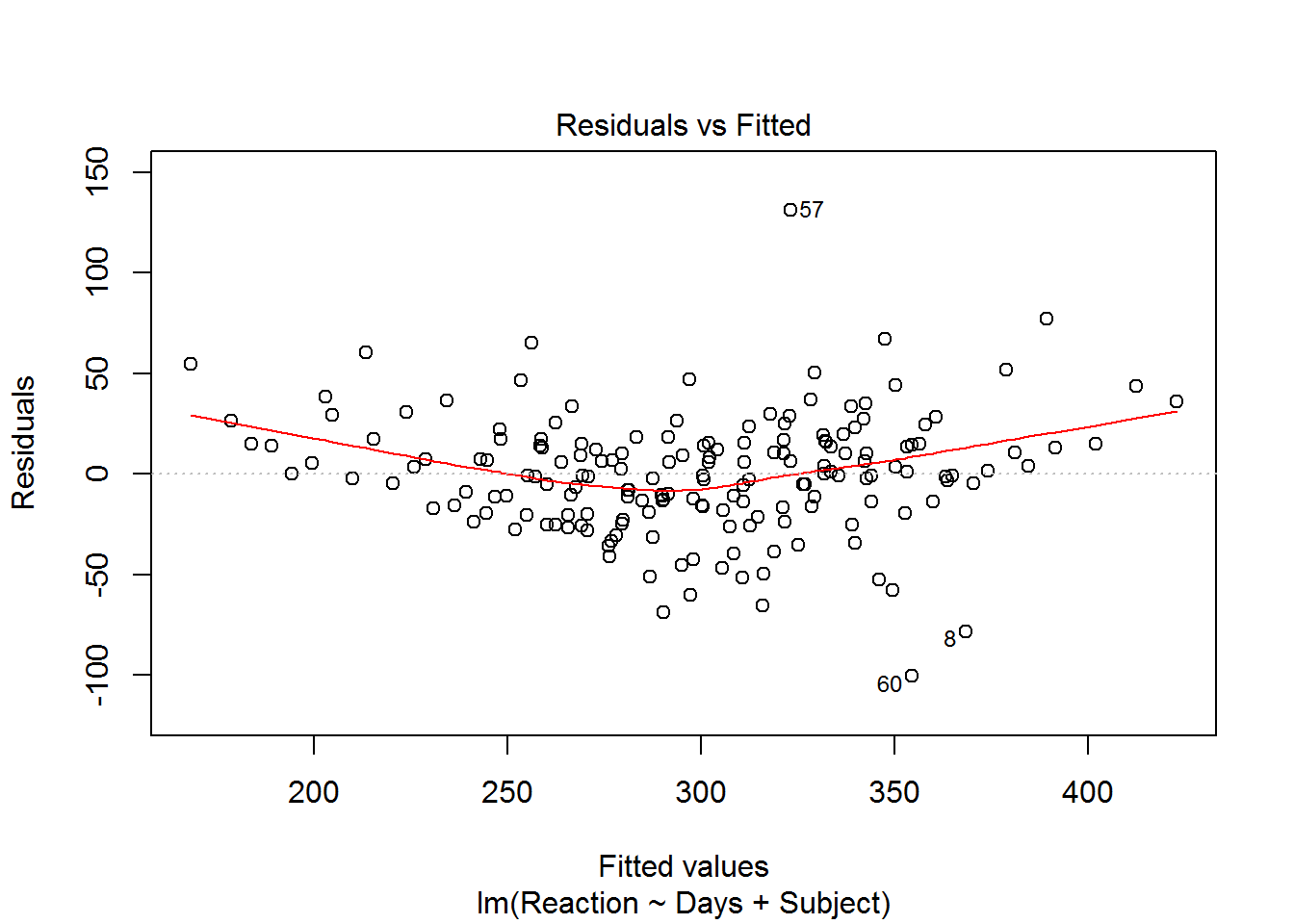
```
```
plot(mod, which = 2)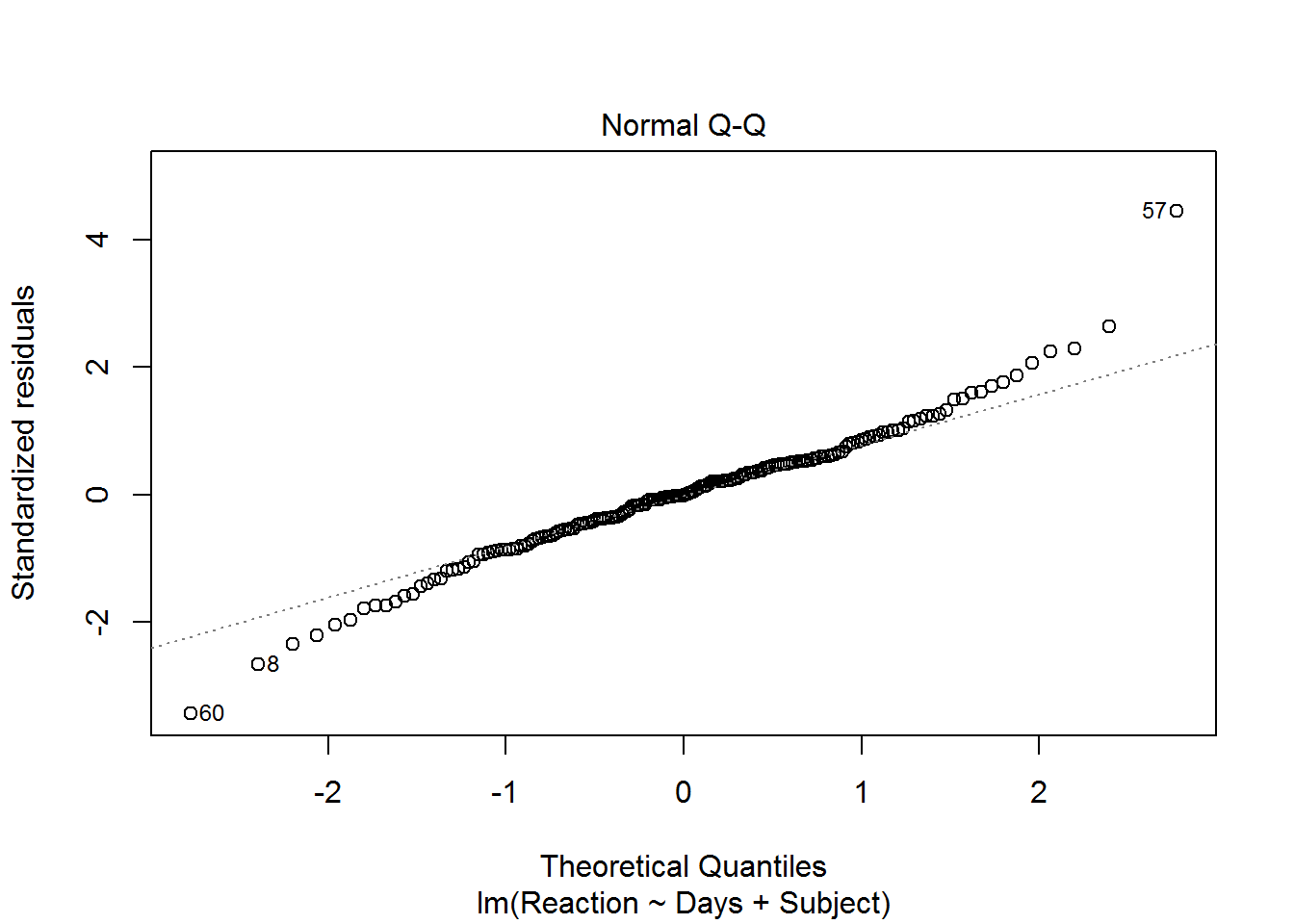
```
```
plot(mod, which = 5)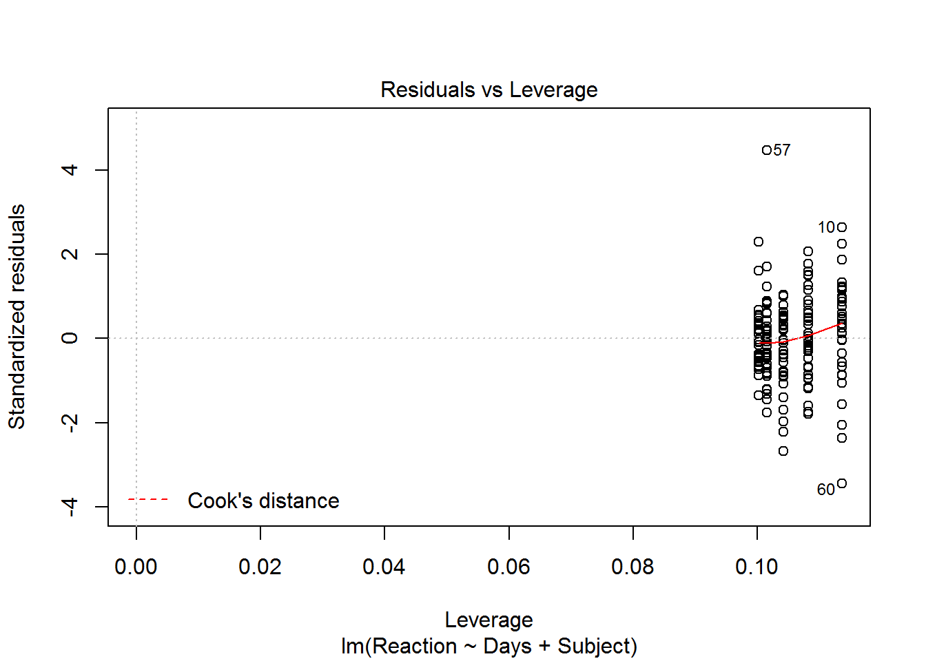
```

Results

summary() function

The summary() function provides a nice summary of a model object. You could also use the str() function to see the details of what is included in the model object.

The following examples display the summary for the three models created above.

Enter the following command in your script and run it.
```
summary(mod)
```

The results of the above command are shown below.


Call:
lm(formula = Reaction ~ Days + Subject, data = sleepstudy)

Residuals:
     Min       1Q   Median       3Q      Max 
-100.540  -16.389   -0.341   15.215  131.159 

Coefficients:
             Estimate Std. Error t value Pr(>|t|)    
(Intercept)  295.0310    10.4471  28.240  < 2e-16 ***
Days          10.4673     0.8042  13.015  < 2e-16 ***
Subject309  -126.9008    13.8597  -9.156 2.35e-16 ***
Subject310  -111.1326    13.8597  -8.018 2.07e-13 ***
Subject330   -38.9124    13.8597  -2.808 0.005609 ** 
Subject331   -32.6978    13.8597  -2.359 0.019514 *  
Subject332   -34.8318    13.8597  -2.513 0.012949 *  
Subject333   -25.9755    13.8597  -1.874 0.062718 .  
Subject334   -46.8318    13.8597  -3.379 0.000913 ***
Subject335   -92.0638    13.8597  -6.643 4.51e-10 ***
Subject337    33.5872    13.8597   2.423 0.016486 *  
Subject349   -66.2994    13.8597  -4.784 3.87e-06 ***
Subject350   -28.5311    13.8597  -2.059 0.041147 *  
Subject351   -52.0361    13.8597  -3.754 0.000242 ***
Subject352    -4.7123    13.8597  -0.340 0.734300    
Subject369   -36.0992    13.8597  -2.605 0.010059 *  
Subject370   -50.4321    13.8597  -3.639 0.000369 ***
Subject371   -47.1498    13.8597  -3.402 0.000844 ***
Subject372   -24.2477    13.8597  -1.750 0.082108 .  
---
Signif. codes:  0 '***' 0.001 '**' 0.01 '*' 0.05 '.' 0.1 ' ' 1

Residual standard error: 30.99 on 161 degrees of freedom
Multiple R-squared:  0.7277,    Adjusted R-squared:  0.6973 
F-statistic: 23.91 on 18 and 161 DF,  p-value: < 2.2e-16

The summary display starts with the call to lm which generated the model object.

The residual summary is the five number summary for the residuals. This can be used as a quick check for skewed residuals.

The coefficient's summary shows the estimated value, standard error, and p-value for each coefficient. The p-values are from Wald tests of each coefficient being equal to zero. For OLS models this is equivalent to an F-test of nested models with the variable of interest being removed in the nested model.

The display ends with information on the model fit. This is the residual standard error, R squared of the model, and the F-test of the significance of the model verse the null model.

Enter the following command in your script and run it.
```
summary(modglm)
```

The results of the above command are shown below.


Call:
glm(formula = volunteer ~ sex + extraversion * neuroticism, family = binomial, 
    data = Cowles)

Deviance Residuals: 
    Min       1Q   Median       3Q      Max  
-1.4749  -1.0602  -0.8934   1.2609   1.9978  

Coefficients:
                          Estimate Std. Error z value Pr(>|z|)    
(Intercept)              -2.358207   0.501320  -4.704 2.55e-06 ***
sexmale                  -0.247152   0.111631  -2.214  0.02683 *  
extraversion              0.166816   0.037719   4.423 9.75e-06 ***
neuroticism               0.110777   0.037648   2.942  0.00326 ** 
extraversion:neuroticism -0.008552   0.002934  -2.915  0.00355 ** 
---
Signif. codes:  0 '***' 0.001 '**' 0.01 '*' 0.05 '.' 0.1 ' ' 1

(Dispersion parameter for binomial family taken to be 1)

    Null deviance: 1933.5  on 1420  degrees of freedom
Residual deviance: 1897.4  on 1416  degrees of freedom
AIC: 1907.4

Number of Fisher Scoring iterations: 4

The summary display for glm models includes similar call, residuls, and coefficient sections. The glm model fit summary includes dispersion, deviance, and iteration information.

Enter the following command in your script and run it.
```
summary(modre)
```
The results of the above command are shown below.
```
Linear mixed model fit by REML ['lmerMod']
Formula: Reaction ~ Days + (Days | Subject)
   Data: sleepstudy

REML criterion at convergence: 1743.6

Scaled residuals: 
    Min      1Q  Median      3Q     Max 
-3.9536 -0.4634  0.0231  0.4634  5.1793 

Random effects:
 Groups   Name        Variance Std.Dev. Corr
 Subject  (Intercept) 612.09   24.740       
          Days         35.07    5.922   0.07
 Residual             654.94   25.592       
Number of obs: 180, groups:  Subject, 18

Fixed effects:
            Estimate Std. Error t value
(Intercept)  251.405      6.825   36.84
Days          10.467      1.546    6.77

Correlation of Fixed Effects:
     (Intr)
Days -0.138
```
The summary display for random effects models includes similar call, residuals, and coefficient sections.

The summary includes a random effects section. This section will display the estimated variances organized by groups. Within each group there will be a row for each random intercept and slope. The variance and standard deviation of the random parameter are provided. The correlation between random effects is also provided when it is estimated. For linear models, the residual is included. For GLM models with defined residuals, such as the logistic and poisson family, no residual information is provided since the model is scaled to the defined error variance.

The glm model fit summary includes convergence information. Here this is REML convergence.

confint() function

The confint() function can be applied to all of the above model object types. The confint() function will calculate a profiled confidence interval when it is appropriate.

The following example displays the confidence intervals for the three models created above.

Enter the following commands in your script and run them.
```
confint(mod)
confint(modglm)
confint(modre)
```

The results of the above command are shown below.

confint(mod)

                  2.5 %    97.5 %
(Intercept)  274.399941 315.66215
Days           8.879103  12.05547
Subject309  -154.271100 -99.53060
Subject310  -138.502810 -83.76231
Subject330   -66.282660 -11.54216
Subject331   -60.068030  -5.32753
Subject332   -62.202010  -7.46151
Subject333   -53.345770   1.39473
Subject334   -74.202030 -19.46153
Subject335  -119.434040 -64.69354
Subject337     6.216930  60.95743
Subject349   -93.669610 -38.92911
Subject350   -55.901400  -1.16090
Subject351   -79.406330 -24.66583
Subject352   -32.082540  22.65796
Subject369   -63.469440  -8.72894
Subject370   -77.802310 -23.06181
Subject371   -74.520040 -19.77954
Subject372   -51.617950   3.12255

confint(modglm)

Waiting for profiling to be done...

                               2.5 %       97.5 %
(Intercept)              -3.35652914 -1.389154923
sexmale                  -0.46642058 -0.028694911
extraversion              0.09374678  0.241771712
neuroticism               0.03744357  0.185227757
extraversion:neuroticism -0.01434742 -0.002833714

confint(modre)

Computing profile confidence intervals ...

                  2.5 %     97.5 %
.sig01       14.3815822  37.715996
.sig02       -0.4815007   0.684986
.sig03        3.8011641   8.753383
.sigma       22.8982669  28.857997
(Intercept) 237.6806955 265.129515
Days          7.3586533  13.575919

predict() function

The predict() function is used to determine the predicted values for a particular set of values of the regressors. The predict() function can also return the confidence interval or prediction interval with the predictions for OLS models.

Syntax and use of the predict() function

predict(modelObj, newObs, interval = intervaltype, level = level, type = type)

The modelObj is an an object returned from a regression function.

The newObs parameter is optional. If it is not provided, the predictions will be for the observed values the model was fit to. The form of newObs is a data.frame with the same columns as used in modelObj.

The intervaltype parameter is available for OLS models. It can be set to "none", "confidence", or "prediction". The default is none, no interval, and alternatively it can be a confidence interval or a prediction interval.

The level parameter is the confidence or prediction level.

The type parameter is used with geralized linear models. The default value is "link", for the linear predictor scale. It can be set to "response" for predictions on the scale of the response variable.

The following example makes predictions for each of the three models from above.

Enter the following commands in your script and run them.

newObs <- data.frame(Days = c(10, 8),
                     Subject = c("331", "372")
                    )
predict(mod, newObs, interval = "prediction")

newObsGlm <- data.frame(sex = c("male"),
                        extraversion = c(8),
                        neuroticism = c(15)
                       )
predict(modglm, newObsGlm, type = "response")

predict(modre, newObs, type = "response")

The results of the above commands are shown below.

newObs <- data.frame(Days = c(10, 8),
                     Subject = c("331", "372")
                    )
predict(mod, newObs, interval = "prediction")

       fit      lwr      upr
1 367.0061 302.2256 431.7867
2 354.5216 290.0925 418.9508

newObsGlm <- data.frame(sex = c("male"),
                        extraversion = c(8),
                        neuroticism = c(15)
                       )
predict(modglm, newObsGlm, type = "response")

        1 
0.3462704

predict(modre, newObs, type = "response")

       1        2 
347.6392 357.7302

Extractors

Extractor functions are the preferred method for retrieving information on the model. Some commonly used extractor functions are listed below.

fitted()

The fitted() function returns the predicted values for the observation in the data set used to fit the model.
residual()

The residual() function returns the residual values from the fitted model.
hatvalues()

The hatvalues() function returns the hat values, leverage measures, that result from fitting the model.
Influence measures

The cooks.distance() and influence() functions returns the Cook's distance or a set of influence measures that resulted from fitting the model.

R - A Brief Introduction to Regression

Specifying a model

Formula

Linear models - Ordinary Least Squares models (OLS)

Generalized linear models (GLM)

Random parameters

Variable selection functions

Diagnostics

Results

summary() function

confint() function

predict() function

Extractors

Further reading