R for Researchers: Regression inference solutions

April 2015

This article contains solutions to exercises for an article in the series R for Researchers. For a list of topics covered by this series, see the Introduction article. If you're new to R we highly recommend reading the articles in order.

There is often more than one approach to the exercises. Do not be concerned if your approach is different than the solution provided.

These solutions require the solutions from the prior lesson be run in your R session.

Exercise solutions

These exercises use the alfalfa dataset and the work you started on the alfAnalysis script. Open the script and run all the commands in the script to prepare your session for these problems.

Note, we will use the shade and irrig variable as continuous variables for these exercise. They could also be considered as factor variables. Since both represent increasing levels we first try to use them as scale.

Find the confidence interval for the model coefficients.

confint(out5)

                 2.5 %      97.5 %
(Intercept) 24.4862967 29.48970330
irrig       -1.0167775 -0.07122252
inocA        4.4856748  8.71432519
inocB        3.7656748  7.99432519
inocC        4.4056748  8.63432519
inocD        3.6256748  7.85432519
shade        0.7952225  1.74077748

Test if inoculant A equals inoculant D.

linearHypothesis(out5,
    c("inocA-inocD") )

Linear hypothesis test

Hypothesis:
inocA - inocD = 0

Model 1: restricted model
Model 2: yield ~ irrig + inoc + shade

  Res.Df    RSS Df Sum of Sq      F Pr(>F)
1     19 47.425                           
2     18 45.576  1     1.849 0.7303  0.404

This data set does not provide evidence that inoculant A and D are different, when considered at the same level of irrigation and shade.

Predict the confidence interval for the mean yield for a plot which has irrigation level 3, shade level 5, and inoculant C.

newAlfObs <- data.frame(irrig=c(3),
                     inoc=c("C"),
                     shade=c(5)
)
predict(out5, newAlfObs, interval="confidence")

     fit      lwr      upr
1 38.216 36.44703 39.98497

Plot the observered verse fitted values for your model

ggplot(out5Diag, aes(x=fit)) +
  geom_point(aes(y=yield, col=inoc)) +
  geom_line(aes(y=fit)) +
  theme_bw() +
  ggtitle("Alfalfa Yields Vs Predicted") +
  theme( plot.title=element_text(vjust=1.0) ) +
  xlab("Predicted Yield") +
  theme( axis.title.x = element_text(vjust=-.5) ) +
  ylab("Observed yield") +
  theme( axis.title.y = element_text(vjust=1.0) ) +
  theme(legend.position = "bottom")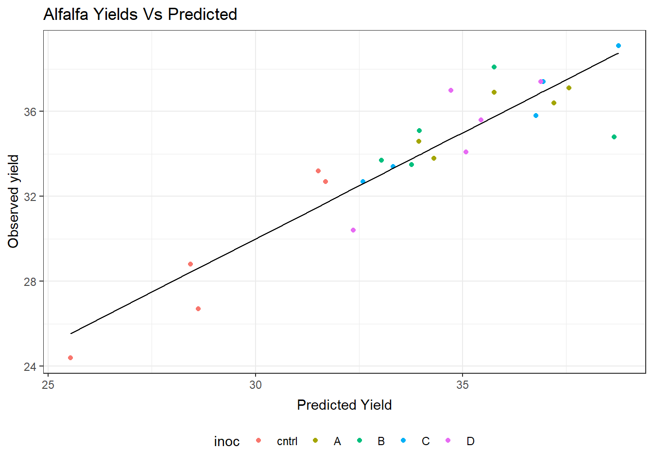

Commit your changes to AlfAnalysis.

Return to the Regression inference article.

Last Revised: 3/9/2015