This article is part of the Multiple Imputation in Stata series. For a list of topics covered by this series, see the Introduction.
This article contains examples that illustrate some of the issues involved in using multiple imputation. Articles in the Multiple Imputation in Stata series refer to these examples, and more discussion of the principles involved can be found in those articles. However, it is possible to read this article independently, or to just read about the particular example that interests you (see the list of examples below).
These examples are not intended to test the validity of the techniques used or rigorously compare their effectiveness. However, they should give you some intuition about how they work and their strengths and weaknesses. Some of the simulation parameters (and occasionally the seed for the random number generator) were chosen in order to highlight the issue at hand, but none of them are atypical of real-world situations. The data are generated randomly from standard distributions in such a way that the "right" answers are known and you can see how closely different techniques approach those answers.
A Stata do file is provided for each example, along with commentary and selected output (in this web page). The do file also generates the data set used, with a set seed for reproducibility. Our suggestion is that you open the do file in Stata's do file editor or your favorite text editor and read it in parallel with the discussion in the article. Please note that the example do files are not intended to demonstrate the entire process of multiple imputation—they don't always check the fit or convergence of the imputation models, for example, which are very important things to do in real world use of multiple imputation.
Each example concludes with a "Lessons Learned" section, but we'd like to highlight one overall lesson: Multiple imputation can be a useful tool, but there are many ways to get it wrong and invalidate your results. Be very careful, and don't expect it to be quick and easy.
The examples are:
- Power
- MCAR vs. MAR vs. MNAR
- Imputing the Dependent Variable
- Non-Normal Data
- Transformations
- Non-Linearity
- Interactions
Power
The most common motivation for using multiple imputation is to try to increase the power of statistical tests by increasing the number of observations used (i.e. by not losing observations due to missing values). In our experience it rarely makes a large difference in practice. This example uses ideal circumstances to illustrate what extremely successful multiple imputation would look like.
Data
Observations: 1,000
Variables:
- x1-x10 drawn from standard normal distribution (independently)
- y is the sum of all x's, plus a normal error term
Missingness: Each value of the x variables has a 10% chance of being missing (MCAR).
Right Answers: Regressing y on all the x's, each x should have a coefficient of 1.
Procedure
Begin with complete cases analysis:
      Source |       SS       df       MS              Number of obs =     369
-------------+------------------------------           F( 10,   358) =    6.71
       Model |  3882.86207    10  388.286207           Prob > F      =  0.0000
    Residual |  20722.7734   358   57.884842           R-squared     =  0.1578
-------------+------------------------------           Adj R-squared =  0.1343
       Total |  24605.6355   368    66.86314           Root MSE      =  7.6082

------------------------------------------------------------------------------
           y |      Coef.   Std. Err.      t    P>|t|     [95% Conf. Interval]
-------------+----------------------------------------------------------------
          x1 |    .733993   .4216582     1.74   0.083    -.0952453    1.563231
          x2 |   1.664231   .3867292     4.30   0.000      .903684    2.424777
          x3 |    1.51406   .3907875     3.87   0.000     .7455327    2.282588
          x4 |   .2801067    .395164     0.71   0.479    -.4970278    1.057241
          x5 |   .8524305   .4076557     2.09   0.037     .0507297    1.654131
          x6 |   .7704437    .413519     1.86   0.063     -.042788    1.583675
          x7 |   .6512155   .3938107     1.65   0.099    -.1232575    1.425689
          x8 |   .9173208   .3969585     2.31   0.021     .1366572    1.697984
          x9 |   .8736406   .4115488     2.12   0.034     .0642835    1.682998
         x10 |   .9222064   .4123417     2.24   0.026       .11129    1.733123
       _cons |  -.1999121   .3975523    -0.50   0.615    -.9817434    .5819192
------------------------------------------------------------------------------
Note that although each x value has just a 10% chance of being missing, because we have ten x variables per observation almost 2/3 of the observations are missing at least one value and must be dropped. As a result, the standard errors are quite large, and the coefficients on four of the ten x's are not significantly different from zero.
After multiple imputation, the same regression gives the following:
Multiple-imputation estimates                     Imputations     =         10
Linear regression                                 Number of obs   =       1000
                                                  Average RVI     =     0.1483
                                                  Largest FMI     =     0.2356
                                                  Complete DF     =        989
DF adjustment:   Small sample                     DF:     min     =     142.63
                                                          avg     =     425.17
                                                          max     =     928.47
Model F test:       Equal FMI                     F(  10,  802.0) =      18.13
Within VCE type:          OLS                     Prob > F        =     0.0000

------------------------------------------------------------------------------
           y |      Coef.   Std. Err.      t    P>|t|     [95% Conf. Interval]
-------------+----------------------------------------------------------------
          x1 |    .793598   .2679515     2.96   0.003     .2657743    1.321422
          x2 |   1.133405   .2482047     4.57   0.000     .6460259    1.620785
          x3 |    1.33182   .2521916     5.28   0.000     .8364684    1.827172
          x4 |   1.159887   .2714759     4.27   0.000      .624309    1.695465
          x5 |   1.181207   .2901044     4.07   0.000      .607747    1.754667
          x6 |   1.305636   .2835268     4.60   0.000     .7466279    1.864645
          x7 |   .6258813   .2568191     2.44   0.015      .121268    1.130494
          x8 |   1.143631    .253376     4.51   0.000     .6461328     1.64113
          x9 |   1.112347   .2838261     3.92   0.000     .5520503    1.672644
         x10 |   1.053309   .2612807     4.03   0.000     .5397648    1.566854
       _cons |   .0305628   .2499378     0.12   0.903    -.4599457    .5210712
------------------------------------------------------------------------------
The standard errors are much smaller than with complete cases analysis, and all of the coefficients are significantly different from zero. This illustrates the primary motivation for using multiple imputation.
Lessons Learned
This data set is ideal for multiple imputation because it has large numbers of observations with partial data. Complete cases analysis must discard all these observations. Multiple imputation can use the information they contain to improve the results.
Note that the imputation model could not do a very good job of predicting the missing values of the x's based on the observed data. The x's are completely independent of each other and thus have no predictive power. y has some but not much: if you regress each x on y and all the other x's (which is what the imputation model used does), the R-squared values are all less than 0.1 and most are less than 0.03. The success of multiple imputation does not depend on imputing the "right" values of the missing variables for individual observations, but rather on correctly modeling their distribution conditional on the observed data.
MCAR vs. MAR vs. MNAR
Whether your data are Missing Completely at Random (probability of being missing does not depend on either observed or unobserved data), Missing at Random (probability of being missing depends only on observed data), or Missing Not at Random (probability of being missing depends on unobserved data) is very important in deciding how to analyze it. This example shows how complete cases analysis and multiple imputation respond to different mechanisms for missingness.
Data
Observations: 1,000
Variables:
- x is drawn from standard normal distribution
- y is x plus a normal error term
Missingness:
- y is always observed
- First run: probability of x being missing is 10% for all observations (MCAR)
- Second run: probability of x being missing is proportional to y (MAR)
- Third run: probability of x being missing is proportional to x (MNAR)
Right Answers: Regressing y on x, x should have a coefficient of 1.
Procedure
We'll analyze this data set three times, once when it is MCAR, once when it is MAR, and once when it is MNAR.
MCAR
In the first run, the data set is MCAR and both complete cases analysis and multiple imputation give unbiased results.
Complete cases analysis:
      Source |       SS       df       MS              Number of obs =     882
-------------+------------------------------           F(  1,   880) =  932.47
       Model |   918.60551     1   918.60551           Prob > F      =  0.0000
    Residual |  866.913167   880  .985128598           R-squared     =  0.5145
-------------+------------------------------           Adj R-squared =  0.5139
       Total |  1785.51868   881  2.02669543           Root MSE      =  .99254

------------------------------------------------------------------------------
           y |      Coef.   Std. Err.      t    P>|t|     [95% Conf. Interval]
-------------+----------------------------------------------------------------
           x |   .9842461   .0322319    30.54   0.000     .9209858    1.047506
       _cons |  -.0481664   .0334249    -1.44   0.150    -.1137683    .0174354
------------------------------------------------------------------------------
Multiple imputation:
Multiple-imputation estimates                     Imputations     =         10
Linear regression                                 Number of obs   =       1000
                                                  Average RVI     =     0.1112
                                                  Largest FMI     =     0.1583
                                                  Complete DF     =        998
DF adjustment:   Small sample                     DF:     min     =     262.51
                                                          avg     =     541.98
                                                          max     =     821.46
Model F test:       Equal FMI                     F(   1,  821.5) =    1014.02
Within VCE type:          OLS                     Prob > F        =     0.0000

------------------------------------------------------------------------------
           y |      Coef.   Std. Err.      t    P>|t|     [95% Conf. Interval]
-------------+----------------------------------------------------------------
           x |   .9837383   .0308928    31.84   0.000     .9231003    1.044376
       _cons |  -.0377668   .0342445    -1.10   0.271    -.1051958    .0296621
------------------------------------------------------------------------------
MAR
Now, consider the case where the probability of x being missing is proportional to y (which is always observed), making the data MAR. With MAR data, complete cases analysis is biased:
      Source |       SS       df       MS              Number of obs =     652
-------------+------------------------------           F(  1,   650) =  375.85
       Model |  252.090968     1  252.090968           Prob > F      =  0.0000
    Residual |  435.966034   650  .670716976           R-squared     =  0.3664
-------------+------------------------------           Adj R-squared =  0.3654
       Total |  688.057002   651   1.0569232           Root MSE      =  .81897

------------------------------------------------------------------------------
           y |      Coef.   Std. Err.      t    P>|t|     [95% Conf. Interval]
-------------+----------------------------------------------------------------
           x |   .6857927    .035374    19.39   0.000     .6163317    .7552538
       _cons |   -.558313   .0352209   -15.85   0.000    -.6274736   -.4891525
------------------------------------------------------------------------------
However, multiple imputation gives unbiased estimates:
Multiple-imputation estimates                     Imputations     =         10
Linear regression                                 Number of obs   =       1000
                                                  Average RVI     =     0.4234
                                                  Largest FMI     =     0.3335
                                                  Complete DF     =        998
DF adjustment:   Small sample                     DF:     min     =      78.63
                                                          avg     =      90.20
                                                          max     =     101.78
Model F test:       Equal FMI                     F(   1,   78.6) =     750.78
Within VCE type:          OLS                     Prob > F        =     0.0000

------------------------------------------------------------------------------
           y |      Coef.   Std. Err.      t    P>|t|     [95% Conf. Interval]
-------------+----------------------------------------------------------------
           x |   .9909115   .0361642    27.40   0.000     .9189232      1.0629
       _cons |  -.0544014   .0366092    -1.49   0.140    -.1270175    .0182146
------------------------------------------------------------------------------
MNAR
Finally consider the case where the probability of x being missing proportional to x. This makes the data missing not at random (MNAR), and with MNAR data both complete cases analysis and multiple imputation are biased.
Complete cases analysis:
      Source |       SS       df       MS              Number of obs =     679
-------------+------------------------------           F(  1,   677) =  463.29
       Model |   464.94386     1   464.94386           Prob > F      =  0.0000
    Residual |  679.422756   677  1.00357866           R-squared     =  0.4063
-------------+------------------------------           Adj R-squared =  0.4054
       Total |  1144.36662   678  1.68785636           Root MSE      =  1.0018

------------------------------------------------------------------------------
           y |      Coef.   Std. Err.      t    P>|t|     [95% Conf. Interval]
-------------+----------------------------------------------------------------
           x |   1.093581   .0508074    21.52   0.000     .9938225     1.19334
       _cons |   .0420364   .0469578     0.90   0.371     -.050164    .1342368
------------------------------------------------------------------------------
Multiple imputation:
Multiple-imputation estimates                     Imputations     =         10
Linear regression                                 Number of obs   =       1000
                                                  Average RVI     =     0.3930
                                                  Largest FMI     =     0.3425
                                                  Complete DF     =        998
DF adjustment:   Small sample                     DF:     min     =      74.96
                                                          avg     =     144.00
                                                          max     =     213.04
Model F test:       Equal FMI                     F(   1,   75.0) =     561.03
Within VCE type:          OLS                     Prob > F        =     0.0000

------------------------------------------------------------------------------
           y |      Coef.   Std. Err.      t    P>|t|     [95% Conf. Interval]
-------------+----------------------------------------------------------------
           x |   1.223772   .0516665    23.69   0.000     1.120846    1.326698
       _cons |   .3816984   .0402614     9.48   0.000     .3023366    .4610602
------------------------------------------------------------------------------
Complete cases analysis actually does better with this particular data set, but that's not true in general.
Lessons Learned
Always investigate whether your data set is plausibly MCAR or MAR. (For example, run logits on indicators of missingness and see if anything predicts it—if it does the data set is MAR rather than MCAR.) If your data set is MAR, consider using multiple imputation rather than complete cases analysis.
MNAR, by definition, cannot be detected by looking at the observed data. You'll have to think carefully about how the data was collected and consider whether some values of the variables might make the data more or less likely to be observed. Unfortunately, the options for working with MNAR data are limited.
Imputing the Dependent Variable
Many researchers believe it is inappropriate to use imputed values of the dependent variable in the analysis model, especially if the variables used in the imputation model are the same as the variables used in the analysis model. The thinking is that the imputed values add no information since they were generated using the model that is being analyzed.
Unfortunately, this sometimes is misunderstood as meaning that the dependent variable should not be included in the imputation model. That would be a major mistake.
Complete code for this example
Data
Observations: 1,000
Variables:
- x1-x3 drawn from standard normal distribution (independently)
- y is the sum of all x's, plus a normal error term
Missingness: y and x1-x3 have a 20% probability of being missing (MCAR).
Right Answers: Regressing y on x1-x3, the coefficient on each should be 1.
Procedure
The following are the results of complete cases analysis:
      Source |       SS       df       MS              Number of obs =    4079
-------------+------------------------------           F(  3,  4075) = 3944.41
       Model |  12264.8582     3  4088.28608           Prob > F      =  0.0000
    Residual |  4223.63457  4075  1.03647474           R-squared     =  0.7438
-------------+------------------------------           Adj R-squared =  0.7437
       Total |  16488.4928  4078  4.04327926           Root MSE      =  1.0181

------------------------------------------------------------------------------
           y |      Coef.   Std. Err.      t    P>|t|     [95% Conf. Interval]
-------------+----------------------------------------------------------------
          x1 |   .9834974   .0160921    61.12   0.000     .9519481    1.015047
          x2 |   1.000172   .0160265    62.41   0.000     .9687511    1.031593
          x3 |   1.003089   .0159724    62.80   0.000     .9717744    1.034404
       _cons |  -.0003362   .0159445    -0.02   0.983    -.0315962    .0309238
------------------------------------------------------------------------------
If you leave y out of the imputation model, imputing only x1-x3, the coefficients on the x's in the final model are biased towards zero:
Multiple-imputation estimates                     Imputations     =         10
Linear regression                                 Number of obs   =       7993
                                                  Average RVI     =     0.4014
                                                  Largest FMI     =     0.3666
                                                  Complete DF     =       7989
DF adjustment:   Small sample                     DF:     min     =      72.62
                                                          avg     =     119.53
                                                          max     =     161.84
Model F test:       Equal FMI                     F(   3,  223.0) =    1761.75
Within VCE type:          OLS                     Prob > F        =     0.0000

------------------------------------------------------------------------------
           y |      Coef.   Std. Err.      t    P>|t|     [95% Conf. Interval]
-------------+----------------------------------------------------------------
          x1 |   .7946113   .0185175    42.91   0.000     .7580219    .8312007
          x2 |   .7983325   .0199962    39.92   0.000     .7584766    .8381885
          x3 |   .8001109   .0193738    41.30   0.000     .7616436    .8385782
       _cons |   .0041643   .0183891     0.23   0.821    -.0321492    .0404778
------------------------------------------------------------------------------
Why is that? An easy way to see the problem is to look at correlations. First, the correlation between y and x1 in the unimputed data:
            |        y       x1
-------------+------------------
           y |   1.0000
          x1 |   0.5032   1.0000
Now, the correlation between y and x1 for those observations where x1 is imputed (this is calculated for the first imputation, but the others are similar):
             |        y       x1
-------------+------------------
           y |   1.0000
          x1 |  -0.0073   1.0000
Because y is not included in the imputation model, the imputation model creates values of x1 (and x2 and x3) which are not correlated with y. This does not match the observed data. It also biases the results of the final model by adding observations in which y really is unrelated to x1, x2, and x3.
This problem goes away if y is included in the imputation model. Given the nature of chained equations, this means that values of y must be imputed. However, you're under no obligation to use those values in your analysis model. Simply create an indicator variable for "y is missing in the observed data," which can be done automatically with misstable sum, gen(miss_), and then add if !miss_y to the regression command. This restricts the regression to those observations where y is actually observed, so any imputed values of y are not used. Here are the results:
Multiple-imputation estimates                     Imputations     =         10
Linear regression                                 Number of obs   =       7993
                                                  Average RVI     =     0.6402
                                                  Largest FMI     =     0.5076
                                                  Complete DF     =       7989
DF adjustment:   Small sample                     DF:     min     =      38.27
                                                          avg     =      82.39
                                                          max     =     182.83
Model F test:       Equal FMI                     F(   3,  137.9) =    4691.72
Within VCE type:          OLS                     Prob > F        =     0.0000

------------------------------------------------------------------------------
           y |      Coef.   Std. Err.      t    P>|t|     [95% Conf. Interval]
-------------+----------------------------------------------------------------
          x1 |   .9852388   .0150348    65.53   0.000     .9550372     1.01544
          x2 |   .9923264   .0158077    62.77   0.000     .9603327     1.02432
          x3 |   .9936324   .0129186    76.91   0.000     .9681437    1.019121
       _cons |  -.0015309   .0145755    -0.11   0.917    -.0306997    .0276378
------------------------------------------------------------------------------
On the other hand, using the imputed values of y turns out to make almost no difference in this case (see the complete code).
Lessons Learned
Always include the dependent variable in your imputation model. Whether you should use imputed values of the dependent variable in your analysis model is unclear, but always impute them.
Non-Normal Data
The obvious way to impute a continuous variable is regression (i.e. the regress command in mi impute chained). However, it applies a normal error term. What happens if a variable is not at all normally distributed?
Complete code for this example
Data
Observations: 10,000
Variables:
- g is a binary (1/0) variable with a 50% probability of being 1
- x is drawn from the standard normal distribution, then 5 is added if g is 1. Thus x is bimodal.
- y is x plus a normal error term
Missingness: Both y and x have a 10% probability of being missing (MCAR).
Right Answers: Regressing y on x, x should have a coefficient of 1.
Procedure
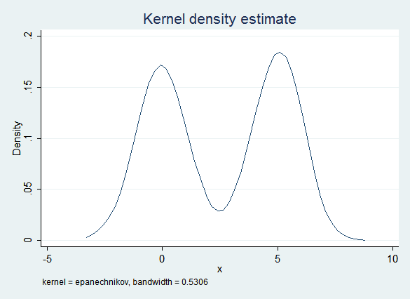
Given the way x was constructed, it has a bimodal distribution and is definitely not normal:

The obvious imputation model (regress x on y) captures some of this bimodality because of the influence of y. However, the error term is normal and does not take into account the non-normal distribution of the data. Thus this model is too likely to create imputed values that are near 2.5 (the "valley" between the two "peaks") and the distribution of the imputed data is "too normal":
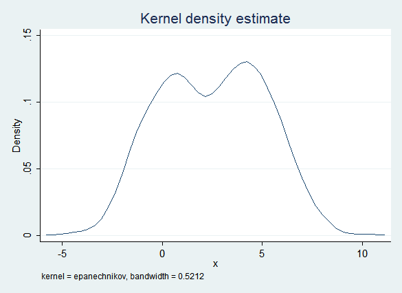
However, the regression results are quite good:
Multiple-imputation estimates                     Imputations     =         10
Linear regression                                 Number of obs   =      10000
                                                  Average RVI     =     0.2471
                                                  Largest FMI     =     0.1977
                                                  Complete DF     =       9998
DF adjustment:   Small sample                     DF:     min     =     238.92
                                                          avg     =     414.68
                                                          max     =     590.43
Model F test:       Equal FMI                     F(   1,  590.4) =   63916.86
Within VCE type:          OLS                     Prob > F        =     0.0000

------------------------------------------------------------------------------
           y |      Coef.   Std. Err.      t    P>|t|     [95% Conf. Interval]
-------------+----------------------------------------------------------------
           x |   1.001225   .0039603   252.82   0.000     .9934473    1.009003
       _cons |  -.0068119   .0152489    -0.45   0.655    -.0368514    .0232276
------------------------------------------------------------------------------
Replacing regression with Predictive Mean Matching gives a much better fit. PMM begins with regression, but it then finds the observed value of x that is the nearest match. Because there are fewer observed values in the "valley" PMM is less likely to find a match there, resulting in a distribution that is closer to the original:
Regression results after imputing with PMM are also good:
Multiple-imputation estimates                     Imputations     =         10
Linear regression                                 Number of obs   =      10000
                                                  Average RVI     =     0.2885
                                                  Largest FMI     =     0.2698
                                                  Complete DF     =       9998
DF adjustment:   Small sample                     DF:     min     =     131.79
                                                          avg     =     148.15
                                                          max     =     164.50
Model F test:       Equal FMI                     F(   1,  131.8) =   53733.02
Within VCE type:          OLS                     Prob > F        =     0.0000

------------------------------------------------------------------------------
           y |      Coef.   Std. Err.      t    P>|t|     [95% Conf. Interval]
-------------+----------------------------------------------------------------
           x |   .9976108   .0043037   231.80   0.000     .9890976    1.006124
       _cons |   .0105094   .0156034     0.67   0.502    -.0202993    .0413181
------------------------------------------------------------------------------
On the other hand, x is distributed normally within each g group. If you impute the two groups separately then ordinary regression fits the data quite well:

The regression results are also good:
Multiple-imputation estimates                     Imputations     =         10
Linear regression                                 Number of obs   =      10000
                                                  Average RVI     =     0.6503
                                                  Largest FMI     =     0.4656
                                                  Complete DF     =       9998
DF adjustment:   Small sample                     DF:     min     =      45.53
                                                          avg     =      63.49
                                                          max     =      81.45
Model F test:       Equal FMI                     F(   1,   81.4) =   48664.75
Within VCE type:          OLS                     Prob > F        =     0.0000

------------------------------------------------------------------------------
           y |      Coef.   Std. Err.      t    P>|t|     [95% Conf. Interval]
-------------+----------------------------------------------------------------
           x |   .9996345   .0045314   220.60   0.000     .9906191     1.00865
       _cons |   .0032657   .0183149     0.18   0.859    -.0336105    .0401419
------------------------------------------------------------------------------
Lessons Learned
PMM can be a very effective tool for imputing non-normal data. On the other hand, if you can identify groups whose data may vary in systematically different ways, consider imputing them separately.
However, the regression results were uniformly good, even when the data were imputed using the original regression model where the distribution of the imputed values didn't match the distribution of the observed values very well. In part this is because we had a large number of observations and a simple model, but in general the relationship between face validity and getting valid estimates using the imputed data is unclear.
Transformations
Given non-normal data, it's appealing to try to transform it in a way that makes it more normal. But what if the other variables in the model are related to the original values of the variable rather than the transformed values?
Complete code for this example
Data
Observations: 10,000
Variables:
- x1 is drawn from the standard normal distribution, then exponentiated. Thus it is log-normal
- x2 is drawn from the standard normal distribution
- y is the sum of x1, x2 and a normal error term
Missingness: x1, x2 and y have a 10% probability of being missing (MCAR)
Right Answers: Regressing y on x1 and x2, both should have a coefficient of 1.
Procedure
First, complete cases analysis for comparison. It does quite well, as we'd expect with MCAR data (and a simple model with lots of observations):
      Source |       SS       df       MS              Number of obs =    7299
-------------+------------------------------           F(  2,  7296) =19024.33
       Model |  38421.4045     2  19210.7023           Prob > F      =  0.0000
    Residual |  7367.47472  7296  1.00979643           R-squared     =  0.8391
-------------+------------------------------           Adj R-squared =  0.8391
       Total |  45788.8793  7298  6.27416816           Root MSE      =  1.0049

------------------------------------------------------------------------------
           y |      Coef.   Std. Err.      t    P>|t|     [95% Conf. Interval]
-------------+----------------------------------------------------------------
          x1 |   1.001594   .0057231   175.01   0.000     .9903751    1.012813
          x2 |   .9973623   .0117407    84.95   0.000     .9743471    1.020377
       _cons |   .0035444   .0149663     0.24   0.813     -.025794    .0328827
------------------------------------------------------------------------------
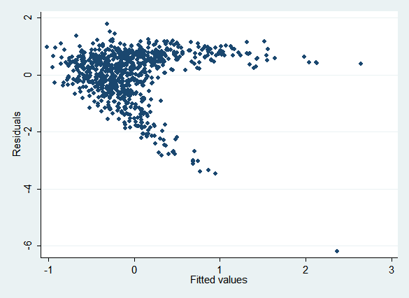
This data set presents a dilemma for imputation: x1 can be made normal simply by taking its log, but y is related to x1, not the log of x1. Regressing ln(x1) on x2 and y (as the obvious imputation model will do) results in the following plot of residuals vs. fitted values (rvfplot):
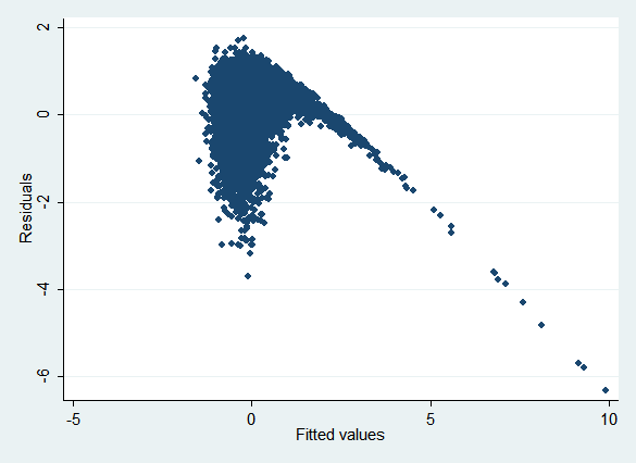
If the model were specified correctly, we'd expect the points to be randomly distributed around the y axis regardless of their x location. Clearly that's not the case.
The obvious way to impute this data would be to:
- Log transform x1 by creating lnx1 = ln(x1)
- Impute lnx1 using regression
- Create the passive variable ix1 = exp(lnx1) to reverse the transformation
Here are the regression results after doing so:
Multiple-imputation estimates                     Imputations     =         10
Linear regression                                 Number of obs   =      10000
                                                  Average RVI     =   196.4421
                                                  Largest FMI     =     0.9987
                                                  Complete DF     =       9997
DF adjustment:   Small sample                     DF:     min     =       5.89
                                                          avg     =     242.41
                                                          max     =     701.09
Model F test:       Equal FMI                     F(   2,   12.8) =       3.84
Within VCE type:          OLS                     Prob > F        =     0.0493

------------------------------------------------------------------------------
           y |      Coef.   Std. Err.      t    P>|t|     [95% Conf. Interval]
-------------+----------------------------------------------------------------
         ix1 |    .014417   .0213705     0.67   0.525    -.0381112    .0669452
          x2 |   .9951566   .0235333    42.29   0.000     .9489525    1.041361
       _cons |   1.583044   .0384844    41.13   0.000     1.502835    1.663253
------------------------------------------------------------------------------
As you see, the coefficient on ix1 (imputed untransformed x1) is very strongly biased towards zero. Now try imputing lnx1 using Predictive Mean Matching rather than regression:
Multiple-imputation estimates                     Imputations     =         10
Linear regression                                 Number of obs   =      10000
                                                  Average RVI     =     0.7058
                                                  Largest FMI     =     0.6292
                                                  Complete DF     =       9997
DF adjustment:   Small sample                     DF:     min     =      24.80
                                                          avg     =      53.56
                                                          max     =      74.84
Model F test:       Equal FMI                     F(   2,   52.8) =    8286.63
Within VCE type:          OLS                     Prob > F        =     0.0000

------------------------------------------------------------------------------
           y |      Coef.   Std. Err.      t    P>|t|     [95% Conf. Interval]
-------------+----------------------------------------------------------------
         ix1 |   .9554301    .009311   102.61   0.000     .9362457    .9746144
          x2 |   .9537128   .0146582    65.06   0.000     .9245112    .9829144
       _cons |   .0843407   .0192948     4.37   0.000     .0457588    .1229226
------------------------------------------------------------------------------
Now both coefficients are biased towards zero, though not nearly as strongly.
What if we simply ignore the fact that x1 is not normally distributed and impute it directly? The results are actually better:
Multiple-imputation estimates                     Imputations     =         10
Linear regression                                 Number of obs   =      10000
                                                  Average RVI     =     0.3873
                                                  Largest FMI     =     0.3401
                                                  Complete DF     =       9997
DF adjustment:   Small sample                     DF:     min     =      84.25
                                                          avg     =     179.94
                                                          max     =     337.16
Model F test:       Equal FMI                     F(   2,  133.4) =   17538.58
Within VCE type:          OLS                     Prob > F        =     0.0000

------------------------------------------------------------------------------
           y |      Coef.   Std. Err.      t    P>|t|     [95% Conf. Interval]
-------------+----------------------------------------------------------------
          x1 |   .9980159   .0060605   164.68   0.000     .9859646    1.010067
          x2 |   .9912113   .0117879    84.09   0.000      .967869    1.014554
       _cons |   .0108679   .0140238     0.77   0.439    -.0167172     .038453
------------------------------------------------------------------------------
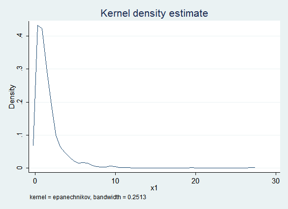
This clearly works well, but raises the question of face validity. Here is a kernel density plot of the observed values of x1:
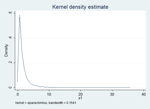
Here is a kernel density plot of the imputed values of x1:
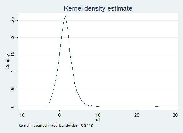
The obvious problem is that the imputed values of x1 are frequently less than zero while the observed values of x1 are always positive. This would be especially problematic if you thought you might want to use a log transform later in the process.
Given the constraint that x1 cannot be less than zero, truncreg seems like a plausible alternative. Unfortunately, truncreg fails to converge for this data set (for reasons not yet clear to us). But PMM will also honor that constraint:
Here are the regression results with PMM:
Multiple-imputation estimates                     Imputations     =         10
Linear regression                                 Number of obs   =      10000
                                                  Average RVI     =     0.3702
                                                  Largest FMI     =     0.3664
                                                  Complete DF     =       9997
DF adjustment:   Small sample                     DF:     min     =      72.89
                                                          avg     =     147.11
                                                          max     =     193.33
Model F test:       Equal FMI                     F(   2,  145.1) =   17890.15
Within VCE type:          OLS                     Prob > F        =     0.0000

------------------------------------------------------------------------------
           y |      Coef.   Std. Err.      t    P>|t|     [95% Conf. Interval]
-------------+----------------------------------------------------------------
          x1 |   1.000568   .0056325   177.64   0.000     .9894588    1.011677
          x2 |   .9977033    .012447    80.16   0.000     .9728958    1.022511
       _cons |    .009171    .014612     0.63   0.531    -.0196674    .0380094
------------------------------------------------------------------------------
Lessons Learned
The lesson of this example is not that you should never transform covariates. Keep in mind that what makes transforming x1 problematic in this example is that the relationship between y and x1 is known to be linear.
The real lesson is that misspecification in your imputation model can cause problems in your analysis model. Be sure to run the regressions implied by your imputation models separately and check them for misspecification. A secondary lesson is that PMM can work well for non-normal data.
Non-Linearity
Non-linear terms in your analysis model present a major challenge in creating an imputation model, because the non-linear relationship between variables can't be easily inverted.
Note: in this example we'll frequently use Stata's syntax for interactions to create squared terms. A varlist of c.x##c.x is equivalent to the varlist x x2 where x2 is defined by gen x2=x^2. The squared term shows up in the output as c.x#c.x. Using c.x##c.x is convenient because you don't have to create a separate variable, and because in that form post-estimation commands can take into account the fact that x and x^2 are not independent variables.
Complete code for this example
Data
Observations: 1,000
Variables:
- x is drawn from the standard normal distribution
- y is x plus x^2 plus a normal error term
Missingness: y and x have a 10% probability of being missing (MCAR).
Right Answers: Regressing y on x and x^2, both should have a coefficient of 1.
Procedure
First, complete cases analysis for comparison:
      Source |       SS       df       MS              Number of obs =     815
-------------+------------------------------           F(  2,   812) = 1184.66
       Model |   2350.4449     2  1175.22245           Prob > F      =  0.0000
    Residual |  805.533089   812  .992035824           R-squared     =  0.7448
-------------+------------------------------           Adj R-squared =  0.7441
       Total |  3155.97799   814  3.87712284           Root MSE      =  .99601

------------------------------------------------------------------------------
           y |      Coef.   Std. Err.      t    P>|t|     [95% Conf. Interval]
-------------+----------------------------------------------------------------
           x |   .9798841   .0344861    28.41   0.000     .9121917    1.047577
             |
     c.x#c.x |   .9948393   .0244134    40.75   0.000     .9469185     1.04276
             |
       _cons |  -.0047983   .0429475    -0.11   0.911    -.0890994    .0795029
------------------------------------------------------------------------------
The obvious thing to do is to impute x, then allow x^2 to be a passive function of x (it makes no difference whether you create a variable for x^2 using mi passive or allow Stata to do it for you by putting c.x##c.x in your regression). However, this means that the imputation model for x simply regresses x on y. This is misspecified, as you can see from an rvfplot:
Here are the regression results. Because the imputation model is misspecified , the coefficient on x^2 (c.x#c.x) is biased:
Multiple-imputation estimates                     Imputations     =         10
Linear regression                                 Number of obs   =       1000
                                                  Average RVI     =     0.9729
                                                  Largest FMI     =     0.5328
                                                  Complete DF     =        997
DF adjustment:   Small sample                     DF:     min     =      32.79
                                                          avg     =      37.89
                                                          max     =      46.68
Model F test:       Equal FMI                     F(   2,   50.2) =     351.77
Within VCE type:          OLS                     Prob > F        =     0.0000

------------------------------------------------------------------------------
           y |      Coef.   Std. Err.      t    P>|t|     [95% Conf. Interval]
-------------+----------------------------------------------------------------
           x |   .9586506   .0570451    16.81   0.000     .8427484    1.074553
             |
     c.x#c.x |    .844537   .0409527    20.62   0.000     .7611974    .9278765
             |
       _cons |   .1986436   .0662195     3.00   0.004     .0654027    .3318845
------------------------------------------------------------------------------
Next impute x using PMM. It's an improvement but still biased:
Multiple-imputation estimates                     Imputations     =         10
Linear regression                                 Number of obs   =       1000
                                                  Average RVI     =     0.3974
                                                  Largest FMI     =     0.3984
                                                  Complete DF     =        997
DF adjustment:   Small sample                     DF:     min     =      56.92
                                                          avg     =     101.37
                                                          max     =     134.94
Model F test:       Equal FMI                     F(   2,  167.9) =     763.23
Within VCE type:          OLS                     Prob > F        =     0.0000

------------------------------------------------------------------------------
           y |      Coef.   Std. Err.      t    P>|t|     [95% Conf. Interval]
-------------+----------------------------------------------------------------
           x |   .9511347    .041403    22.97   0.000     .8691019    1.033167
             |
     c.x#c.x |   .9170003    .027871    32.90   0.000     .8618798    .9721207
             |
       _cons |   .1160666   .0565846     2.05   0.045     .0027546    .2293787
------------------------------------------------------------------------------
The include() option of mi impute chained is usually used to add variables to the imputation model of an individual variable, but it can also accept expressions. Does adding x^2 to the imputation for y with (regress, include((x^2))) y fix the problem? Unfortunately not, though it helps:
Multiple-imputation estimates                     Imputations     =         10
Linear regression                                 Number of obs   =       1000
                                                  Average RVI     =     1.1210
                                                  Largest FMI     =     0.7256
                                                  Complete DF     =        997
DF adjustment:   Small sample                     DF:     min     =      17.48
                                                          avg     =      70.29
                                                          max     =     118.18
Model F test:       Equal FMI                     F(   2,   39.1) =     377.13
Within VCE type:          OLS                     Prob > F        =     0.0000

------------------------------------------------------------------------------
           y |      Coef.   Std. Err.      t    P>|t|     [95% Conf. Interval]
-------------+----------------------------------------------------------------
           x |   .9629371   .0452655    21.27   0.000     .8727678    1.053106
             |
     c.x#c.x |   .8874316   .0475562    18.66   0.000     .7873051    .9875581
             |
       _cons |    .125851    .053619     2.35   0.021     .0196724    .2320296
------------------------------------------------------------------------------
The imputation model for y has been fixed, but the imputation model for x is still misspecified and this still biases the results of the analysis model. Unfortunately, the true dependence of x on y does not match any standard regression model.
Next we'll use what White, Royston and Wood (Multiple imputation using chained equations: Issues and guidance for practice, Statistics in Medicine, November 2010) call the "Just Another Variable" approach. This creates a variable to contain x^2 (x2) and then imputes both x and x2 as if x2 were "just another variable" rather than being determined by x. The obvious disadvantage is that in the imputed data x2 is not equal to x^2, so it lacks face validity. But the regression results are a huge improvement:
Multiple-imputation estimates                     Imputations     =         10
Linear regression                                 Number of obs   =       1000
                                                  Average RVI     =     0.2375
                                                  Largest FMI     =     0.3033
                                                  Complete DF     =        997
DF adjustment:   Small sample                     DF:     min     =      92.98
                                                          avg     =     331.43
                                                          max     =     610.11
Model F test:       Equal FMI                     F(   2,  496.2) =    1330.20
Within VCE type:          OLS                     Prob > F        =     0.0000

------------------------------------------------------------------------------
           y |      Coef.   Std. Err.      t    P>|t|     [95% Conf. Interval]
-------------+----------------------------------------------------------------
           x |   .9905117   .0324469    30.53   0.000     .9267905    1.054233
          x2 |   1.005361   .0240329    41.83   0.000     .9580613    1.052662
       _cons |  -.0018354    .046395    -0.04   0.969    -.0939669    .0902961
------------------------------------------------------------------------------
So would imputing x and x2 using PMM be even better on the theory that PMM is better in sticky situations of all sorts? Not this time:
Multiple-imputation estimates                     Imputations     =         10
Linear regression                                 Number of obs   =       1000
                                                  Average RVI     =     0.3068
                                                  Largest FMI     =     0.3151
                                                  Complete DF     =        997
DF adjustment:   Small sample                     DF:     min     =      86.95
                                                          avg     =     201.95
                                                          max     =     312.22
Model F test:       Equal FMI                     F(   2,  163.9) =    1138.59
Within VCE type:          OLS                     Prob > F        =     0.0000

------------------------------------------------------------------------------
           y |      Coef.   Std. Err.      t    P>|t|     [95% Conf. Interval]
-------------+----------------------------------------------------------------
           x |   .9761798   .0346402    28.18   0.000     .9078863    1.044473
          x2 |   .9987715   .0258422    38.65   0.000      .947407    1.050136
       _cons |  -.0032279   .0416431    -0.08   0.938    -.0851645    .0787087
------------------------------------------------------------------------------
Lessons Learned
Again, the principal lesson is that misspecification in your imputation model can lead to bias in your analysis model. Be very careful, and always check the fit of your imputation models.
This is a continuing research area, but there appears to be some agreement that imputing non-linear terms as passive variables should be avoided. "Just Another Variable" seems to be a good alternative.
Interactions
Interaction terms in your analysis model also lead to challenges in creating an imputation model because it should take into account the interaction in the model for the covariates being interacted.
Note: we'll again use Stata's syntax for interactions. Putting g##c.x in the covariate list of a regression regresses the dependent variable on g, continuous variable x, and the interaction between g and x. The interaction term shows up in the output as g#c.x.
Complete code for this example
Data
Observations: 10,000
Variables:
- g is a binary (1/0) variable with a 50% probability of being 1
- x is drawn from the standard normal distribution
- y is x plus x*g plus a normal error term. Put differently, y is x plus a normal error term for group 0 and 2*x plus a normal error term for group 1.
Missingness: y and x have a 20% probability of being missing (MCAR).
Right Answers: Regressing y on x, g, and the interaction between x and g, the coefficients for x and the interaction term should be 1, and the coefficient on g should be 0.
Procedure
The following are the results of complete cases analysis:
      Source |       SS       df       MS              Number of obs =    6337
-------------+------------------------------           F(  3,  6333) = 5435.30
       Model |  16167.6705     3   5389.2235           Prob > F      =  0.0000
    Residual |  6279.30945  6333  .991522099           R-squared     =  0.7203
-------------+------------------------------           Adj R-squared =  0.7201
       Total |    22446.98  6336   3.5427683           Root MSE      =  .99575

------------------------------------------------------------------------------
           y |      Coef.   Std. Err.      t    P>|t|     [95% Conf. Interval]
-------------+----------------------------------------------------------------
         1.g |   -.012915   .0250189    -0.52   0.606    -.0619605    .0361305
           x |   .9842869    .017752    55.45   0.000     .9494869    1.019087
             |
       g#c.x |
          1  |   1.026204   .0249124    41.19   0.000     .9773671    1.075041
             |
       _cons |  -.0195648   .0177789    -1.10   0.271    -.0544175    .0152879
------------------------------------------------------------------------------
The obvious way to impute this data is to impute x and create the interaction term passively. However that means x is regressed on y and g without any interactions. The result is biased estimates (in opposite directions) of the coefficients for both x and the interaction term:
Multiple-imputation estimates                     Imputations     =         10
Linear regression                                 Number of obs   =      10000
                                                  Average RVI     =     0.5760
                                                  Largest FMI     =     0.3048
                                                  Complete DF     =       9996
DF adjustment:   Small sample                     DF:     min     =     104.17
                                                          avg     =     130.43
                                                          max     =     182.89
Model F test:       Equal FMI                     F(   3,  205.4) =    4870.03
Within VCE type:          OLS                     Prob > F        =     0.0000

------------------------------------------------------------------------------
           y |      Coef.   Std. Err.      t    P>|t|     [95% Conf. Interval]
-------------+----------------------------------------------------------------
         1.g |  -.0077291   .0251103    -0.31   0.759    -.0575089    .0420506
           x |   1.119861   .0182704    61.29   0.000     1.083631    1.156091
             |
       g#c.x |
          1  |   .7300249   .0239816    30.44   0.000     .6827087     .777341
             |
       _cons |  -.0148091   .0174857    -0.85   0.399    -.0494078    .0197896
------------------------------------------------------------------------------
An alternative approach is to create a variable for the interaction term, gx, and impute it separately from x (White, Royston and Wood's "Just Another Variable" approach). As in the previous example with a squared term, the obvious disadvantage is that the imputed value of gx will not in fact be g*x for any given observation. However, the results of the analysis model are much better:
Multiple-imputation estimates                     Imputations     =         10
Linear regression                                 Number of obs   =      10000
                                                  Average RVI     =     0.4359
                                                  Largest FMI     =     0.3753
                                                  Complete DF     =       9996
DF adjustment:   Small sample                     DF:     min     =      69.58
                                                          avg     =     111.30
                                                          max     =     210.61
Model F test:       Equal FMI                     F(   3,  223.1) =    5908.62
Within VCE type:          OLS                     Prob > F        =     0.0000

------------------------------------------------------------------------------
           y |      Coef.   Std. Err.      t    P>|t|     [95% Conf. Interval]
-------------+----------------------------------------------------------------
           x |   .9832953   .0159157    61.78   0.000     .9519209     1.01467
          xg |   1.018901   .0239421    42.56   0.000     .9713602    1.066443
           g |  -.0141319   .0247797    -0.57   0.570    -.0635346    .0352709
       _cons |  -.0087754   .0176281    -0.50   0.620    -.0439374    .0263866
------------------------------------------------------------------------------
Another alternative is to impute the two groups separately. This allows x to have the proper relationship with y in both groups. However, it also allows the relationships between other variables to vary between groups. If you know that some relationships do not vary between groups you'll lose some precision by not taking advantage of this knowledge, but in the real world it's rare know such things.
Multiple-imputation estimates                     Imputations     =         10
Linear regression                                 Number of obs   =      10000
                                                  Average RVI     =     0.3627
                                                  Largest FMI     =     0.3482
                                                  Complete DF     =       9996
DF adjustment:   Small sample                     DF:     min     =      80.48
                                                          avg     =     218.72
                                                          max     =     369.37
Model F test:       Equal FMI                     F(   3,  456.6) =    6783.26
Within VCE type:          OLS                     Prob > F        =     0.0000

------------------------------------------------------------------------------
           y |      Coef.   Std. Err.      t    P>|t|     [95% Conf. Interval]
-------------+----------------------------------------------------------------
         1.g |  -.0218404   .0243087    -0.90   0.372    -.0702117    .0265309
           x |   .9869436   .0156451    63.08   0.000     .9561207    1.017766
             |
       g#c.x |
          1  |   1.018534   .0214947    47.39   0.000      .976267    1.060802
             |
       _cons |  -.0076746   .0158825    -0.48   0.629    -.0390027    .0236534
------------------------------------------------------------------------------
Lessons Learned
Once again, the principal lesson is that misspecification in your imputation model can lead to bias in your analysis model. Be very careful, and always check the fit of your imputation models.
This is also an area of ongoing research, but there appears to be some agreement that imputing interaction effects passively is problematic. If your interactions are all a matter of variables having different effects for different groups, imputing each group separately is probably the obvious solution, though "Just Another Variable" also works well. If you have interactions between continuous variables then use "Just Another Variable."
Acknowledgements
Some of these examples follow the discussion in White, Royston, and Wood. ("Multiple imputation using chained equations: Issues and guidance for practice." Statistics in Medicine. 2011.) We highly recommend this article to anyone who is learning to use multiple imputation.
Next: Recommended Readings
Previous: Estimating
Last Revised: 6/21/2012