This is part four of the Multiple Imputation in Stata series. For a list of topics covered by this series, see the Introduction.
This section will talk you through the details of the imputation process. Be sure you've read at least the previous section, Creating Imputation Models, so you have a sense of what issues can affect the validity of your results.
Example Data
To illustrate the process, we'll use a fabricated data set. Unlike those in the examples section, this data set is designed to have some resemblance to real world data.
Do file that creates this data set
The data set as a Stata data file
Observations: 3,000
Variables:
- female (binary)
- race (categorical, three values)
- urban (binary)
- edu (ordered categorical, four values)
- exp (continuous)
- wage (continuous)
Missingness: Each value of all the variables except female has a 10% chance of being missing completely at random, but of course in the real world we won't know that it is MCAR ahead of time. Thus we will check whether it is MCAR or MAR (MNAR cannot be checked by looking at the observed data) using the procedure outlined in Deciding to Impute:
unab numvars: *
unab missvars: urban-wage
misstable sum, gen(miss_)
foreach var of local missvars {
local covars: list numvars - var
display _newline(3) "logit missingness of `var' on `covars'"
logit miss_`var' `covars'
foreach nvar of local covars {
display _newline(3) "ttest of `nvar' by missingness of `var'"
ttest `nvar', by(miss_`var')
}
}
See the log file for results.
Our goal is to regress wages on sex, race, education level, and experience. To see the "right" answers, open the do file that creates the data set and examine the gen command that defines wage.
Complete code for the imputation process can be found in the following do file:
The imputation process creates a lot of output. We'll put highlights in this page, however, a complete log file including the associated graphs can be found here:
Imputation log file with graphs
Each section of this article will have links to the relevant section of the log. Click "back" in your browser to return to this page.
Setting up
The first step in using mi commands is to mi set your data. This is somewhat similar to svyset, tsset, or xtset. The mi set command tells Stata how it should store the additional imputations you'll create. We suggest using the wide format, as it is slightly faster. On the other hand, mlong uses slightly less memory.
To have Stata use the wide data structure, type:
mi set wide
To have Stata use the mlong (marginal long) data structure, type:
mi set mlong
The wide vs. long terminology is borrowed from reshape and the structures are similar. However, they are not equivalent and you would never use reshape to change the data structure used by mi. Instead, type mi convert wide or mi convert mlong (add ,clear if the data have not been saved since the last change).
Most of the time you don't need to worry about how the imputations are stored: the mi commands figure out automatically how to apply whatever you do to each imputation. But if you need to manipulate the data in a way mi can't do for you, then you'll need to learn about the details of the structure you're using. You'll also need to be very, very careful. If you're interested in such things (including the rarely used flong and flongsep formats) run this do file and read the comments it contains while examining the data browser to see what the data look like in each form.
Registering Variables
The mi commands recognize three kinds of variables:
Imputed variables are variables that mi is to impute or has imputed.
Regular variables are variables that mi is not to impute, either by choice or because they are not missing any values.
Passive variables are variables that are completely determined by other variables. For example, log wage is determined by wage, or an indicator for obesity might be determined by a function of weight and height. Interaction terms are also passive variables, though if you use Stata's interaction syntax you won't have to declare them as such. Passive variables are often problematic—the examples on transformations, non-linearity, and interactions show how using them inappropriately can lead to biased estimates.
If a passive variable is determined by regular variables, then it can be treated as a regular variable since no imputation is needed. Passive variables only have to be treated as such if they depend on imputed variables.
Registering a variable tells Stata what kind of variable it is. Imputed variables must always be registered:
mi register imputed varlist
where varlist should be replaced by the actual list of variables to be imputed.
Regular variables often don't have to be registered, but it's a good idea:
mi register regular varlist
Passive variables must be registered:
mi register passive varlist
However, passive variables are more often created after imputing. Do so with mi passive and they'll be registered as passive automatically.
In our example data, all the variables except female need to be imputed. The appropriate mi register command is:
mi register imputed race-wage
(Note that you cannot use * as your varlist even if you have to impute all your variables, because that would include the system variables added by mi set to keep track of the imputation structure.)
Registering female as regular is optional, but a good idea:
mi register regular female
Checking the Imputation Model
Based on the types of the variables, the obvious imputation methods are:
- race (categorical, three values): mlogit
- urban (binary): logit
- edu (ordered categorical, four values): ologit
- exp (continuous): regress
- wage (continuous): regress
female does not need to be imputed, but should be included in the imputation models both because it is in the analysis model and because it's likely to be relevant.
Before proceeding to impute we will check each of the imputation models. Always run each of your imputation models individually, outside the mi impute chained context, to see if they converge and (insofar as it is possible) verify that they are specified correctly.
Code to run each of these models is:
mlogit race i.urban exp wage i.edu i.female
logit urban i.race exp wage i.edu i.female
ologit edu i.urban i.race exp wage i.female
regress exp i.urban i.race wage i.edu i.female
regress wage i.urban i.race exp i.edu i.female
Note that when categorical variables (ordered or not) appear as covariates i. expands them into sets of indicator variables.
As we'll see later, the output of the mi impute chained command includes the commands for the individual models it runs. Thus a useful shortcut, especially if you have a lot of variables to impute, is to set up your mi impute chained command with the dryrun option to prevent it from doing any actual imputing, run it, and then copy the commands from the output into your do file for testing.
Convergence Problems
The first thing to note is that all of these models run successfully. Complex models like mlogit may fail to converge if you have large numbers of categorical variables, because that often leads to small cell sizes. To pin down the cause of the problem, remove most of the variables, make sure the model works with what's left, and then add variables back one at a time or in small groups until it stops working. With some experimentation you should be able to identify the problem variable or combination of variables. At that point you'll have to decide if you can combine categories or drop variables or make other changes in order to create a workable model.
Prefect Prediction
Perfect prediction is another problem to note. The imputation process cannot simply drop the perfectly predicted observations the way logit can. You could drop them before imputing, but that seems to defeat the purpose of multiple imputation. The alternative is to add the augment (or just aug) option to the affected methods. This tells mi impute chained to use the "augmented regression" approach, which adds fake observations with very low weights in such a way that they have a negligible effect on the results but prevent perfect prediction. For details see the section "The issue of perfect prediction during imputation of categorical data" in the Stata MI documentation.
Checking for Misspecification
You should also try to evaluate whether the models are specified correctly. A full discussion of how to determine whether a regression model is specified correctly or not is well beyond the scope of this article, but use whatever tools you find appropriate. Here are some examples:
Residual vs. Fitted Value Plots
For continuous variables, residual vs. fitted value plots (easily done with rvfplot) can be useful—several of the examples use them to detect problems. Consider the plot for experience:
regress exp i.urban i.race wage i.edu i.female
rvfplot
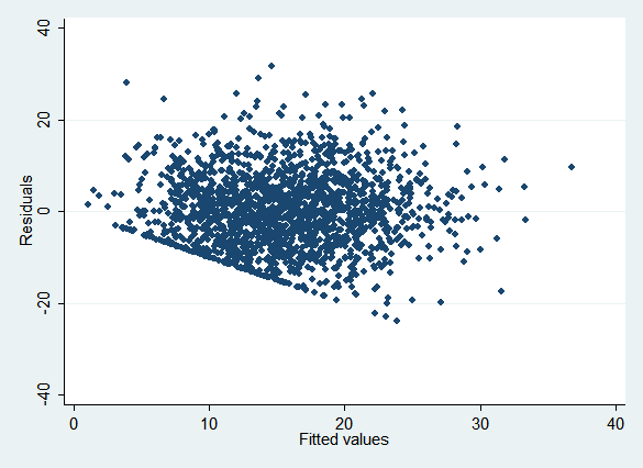
Note how a number of points are clustered along a line in the lower left, and no points are below it:
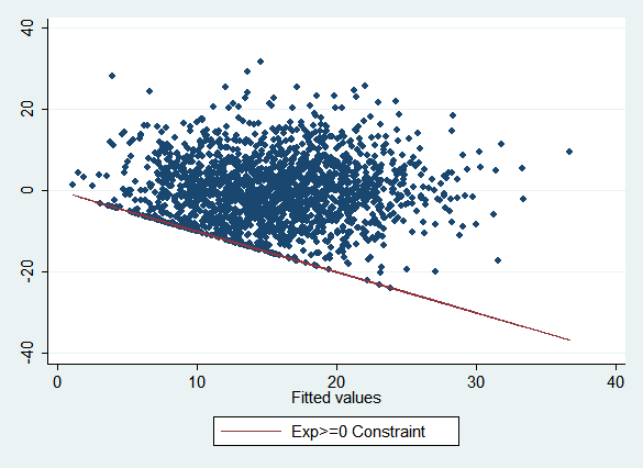
This reflects the constraint that experience cannot be less than zero, which means that the fitted values must always be greater than or equal to the residuals, or alternatively that the residuals must be greater than or equal to the negative of the fitted values. (If the graph had the same scale on both axes, the constraint line would be a 45 degree line.) If all the points were below a similar line rather than above it, this would tell you that there was an upper bound on the variable rather than a lower bound. The y-intercept of the constraint line tells you the limit in either case. You can also have both a lower bound and an upper bound, putting all the points in a band between them.
The "obvious" model, regress, is inappropriate for experience because it won't apply this constraint. It's also inappropriate for wages for the same reason. Alternatives include truncreg, ll(0) and pmm (we'll use pmm).
Adding Interactions
In this example, it seems plausible that the relationships between variables may vary between race, gender, and urban/rural groups. Thus one way to check for misspecification is to add interaction terms to the models and see whether they turn out to be important. For example, we'll compare the obvious model:
regress exp i.race wage i.edu i.urban i.female
with one that includes interactions:
regress exp (i.race i.urban i.female)##(c.wage i.edu)
We'll run similar comparisons for the models of the other variables. This creates a great deal of output, so see the log file for results. Interactions between female and other variables are significant in the models for exp, wage, edu, and urban. There are a few significant interactions between race or urban and other variables, but not nearly as many (and keep in mind that with this many coefficients we'd expect some false positives using a significance level of .05). We'll thus impute the men and women separately. This is an especially good option for this data set because female is never missing. If it were, we'd have to drop those observations which are missing female because they could not be placed in one group or the other.
In the imputation command this means adding the by(female) option. When testing models, it means starting the commands with the by female: prefix (and removing female from the lists of covariates). The improved imputation models are thus:
bysort female: reg exp i.urban i.race wage i.edu
by female: logit urban exp i.race wage i.edu
by female: mlogit race exp i.urban wage i.edu
by female: reg wage exp i.urban i.race i.edu
by female: ologit edu exp i.urban i.race wage
pmm itself cannot be run outside the imputation context, but since it's based on regression you can use regular regression to test it.
These models should be tested again, but we'll omit that process.
Imputing
The basic syntax for mi impute chained is:
mi impute chained (method1) varlist1 (method2) varlist2... = regvars
Each method specifies the method to be used for imputing the following varlist The possibilities for method are regress, pmm, truncreg, intreg, logit, ologit, mlogit, poisson, and nbreg. regvars is a list of regular variables to be used as covariates in the imputation models but not imputed (there may not be any).
The basic options are:
, add(N) rseed(R) savetrace(tracefile, replace)
N is the number of imputations to be added to the data set. R is the seed to be used for the random number generator—if you do not set this you'll get slightly different imputations each time the command is run. The tracefile is a dataset in which mi impute chained will store information about the imputation process. We'll use this dataset to check for convergence.
Options that are relevant to a particular method go with the method, inside the parentheses but following a comma (e.g. (mlogit, aug) ). Options that are relevant to the imputation process as a whole (like by(female) ) go at the end, after the comma.
For our example, the command would be:
mi impute chained (logit) urban (mlogit) race (ologit) edu (pmm) exp wage, add(5) rseed(4409) by(female)
Note that this does not include a savetrace() option. As of this writing, by() and savetrace() cannot be used at the same time, presumably because it would require one trace file for each by group. Stata is aware of this problem and we hope this will be changed soon. For purposes of this article, we'll remove the by() option when it comes time to illustrate use of the trace file. If this problem comes up in your research, talk to us about work-arounds.
Choosing the Number of Imputations
There is some disagreement among authorities about how many imputations are sufficient. Some say 3-10 in almost all circumstances, the Stata documentation suggests at least 20, while White, Royston, and Wood argue that the number of imputations should be roughly equal to the percentage of cases with missing values. However, we are not aware of any argument that increasing the number of imputations ever causes problems (just that the marginal benefit of another imputation asymptotically approaches zero).
Increasing the number of imputations in your analysis takes essentially no work on your part. Just change the number in the add() option to something bigger. On the other hand, it can be a lot of work for the computer—multiple imputation has introduced many researchers into the world of jobs that take hours or days to run. You can generally assume that the amount of time required will be proportional to the number of imputations used (e.g. if a do file takes two hours to run with five imputations, it will probably take about four hours to run with ten imputations). So here's our suggestion:
- Start with five imputations (the low end of what's broadly considered legitimate).
- Work on your research project until you're reasonably confident you have the analysis in its final form. Be sure to do everything with do files so you can run it again at will.
- Note how long the process takes, from imputation to final analysis.
- Consider how much time you have available and decide how many imputations you can afford to run, using the rule of thumb that time required is proportional to the number of imputations. If possible, make the number of imputations roughly equal to the percentage of cases with missing data (a high end estimate of what's required). Allow time to recover if things to go wrong, as they generally do.
- Increase the number of imputations in your do file and start it.
- Do something else while the do file runs, like write your paper. Adding imputations shouldn't change your results significantly—and in the unlikely event that they do, consider yourself lucky to have found that out before publishing.
Speeding up the Imputation Process
Multiple imputation has introduced many researchers into the world of jobs that take hours, days, or even weeks to run. Usually it's not worth spending your time to make Stata code run faster, but multiple imputation can be an exception.
Use the fastest computer available to you. For SSCC members that means learning to run jobs on Linstat, the SSCC's Linux computing cluster. Linux is not as difficult as you may think—Using Linstat has instructions.
Multiple imputation involves more reading and writing to disk than most Stata commands. Sometimes this includes writing temporary files in the current working directory. Use the fastest disk space available to you, both for your data set and for the working directory. In general local disk space will be faster than network disk space, and on Linstat /ramdisk (a "directory" that is actually stored in RAM) will be faster than local disk space. On the other hand, you would not want to permanently store data sets anywhere but network disk space. So consider having your do file do something like the following:
Windows (Winstat or your own PC)
copy x:\mydata\dataset c:\windows\temp\dataset
cd c:\windows\temp
use dataset
{do stuff, including saving results to the network as needed}
erase c:\windows\temp\dataset
Linstat
copy /project/mydata/dataset /ramdisk/dataset
cd /ramdisk
use dataset
{do stuff, including saving results to the network as needed}
erase /ramdisk/dataset
This applies when you're using imputed data as well. If your data set is large enough that working with it after imputation is slow, the above procedure may help.
Checking for Convergence
MICE is an iterative process. In each iteration, mi impute chained first estimates the imputation model, using both the observed data and the imputed data from the previous iteration. It then draws new imputed values from the resulting distributions. Note that as a result, each iteration has some autocorrelation with the previous imputation.
The first iteration must be a special case: in it, mi impute chained first estimates the imputation model for the variable with the fewest missing values based only on the observed data and draws imputed values for that variable. It then estimates the model for the variable with the next fewest missing values, using both the observed values and the imputed values of the first variable, and proceeds similarly for the rest of the variables. Thus the first iteration is often atypical, and because iterations are correlated it can make subsequent iterations atypical as well.
To avoid this, mi impute chained by default goes through ten iterations for each imputed data set you request, saving only the results of the tenth iteration. The first nine iterations are called the burn-in period. Normally this is plenty of time for the effects of the first iteration to become insignificant and for the process to converge to a stationary state. However, you should check for convergence and increase the number of iterations if necessary to ensure it using the burnin() option.
To do so, examine the trace file saved by mi impute chained. It contains the mean and standard deviation of each imputed variable in each iteration. These will vary randomly, but they should not show any trend. An easy way to check is with tsline, but it requires reshaping the data first.
Our preferred imputation model uses by(), so it cannot save a trace file. Thus we'll remove by() for the moment. We'll also increase the burnin() option to 100 so it's easier to see what a stable trace looks like. We'll then use reshape and tsline to check for convergence:
preserve
mi impute chained (logit) urban (mlogit) race (ologit) edu (pmm) exp wage = female, add(5) rseed(88) savetrace(extrace, replace) burnin(100)
use extrace, replace
reshape wide *mean *sd, i(iter) j(m)
tsset iter
tsline exp_mean*, title("Mean of Imputed Values of Experience") note("Each line is for one imputation") legend(off)
graph export conv1.png, replace
tsline exp_sd*, title("Standard Deviation of Imputed Values of Experience") note("Each line is for one imputation") legend(off)
graph export conv2.png, replace
restore
The resulting graphs do not show any obvious problems:
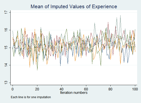
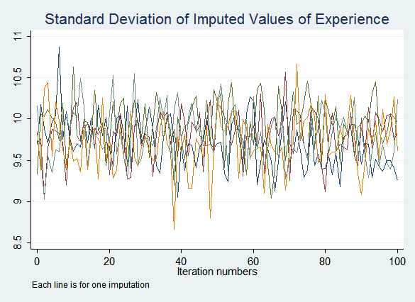
If you do see signs that the process may not have converged after the default ten iterations, increase the number of iterations performed before saving imputed values with the burnin() option. If convergence is never achieved this indicates a problem with the imputation model.
Checking the Imputed Values
After imputing, you should check to see if the imputed data resemble the observed data. Unfortunately there's no formal test to determine what's "close enough." Of course if the data are MAR but not MCAR, the imputed data should be systematically different from the observed data. Ironically, the fewer missing values you have to impute, the more variation you'll see between the imputed data and the observed data (and between imputations).
For binary and categorical variables, compare frequency tables. For continuous variables, comparing means and standard deviations is a good starting point, but you should look at the overall shape of the distribution as well. For that we suggest kernel density graphs or perhaps histograms. Look at each imputation separately rather than pooling all the imputed values so you can see if any one of them went wrong.
mi xeq:
The mi xeq: prefix tell Stata to apply the subsequent command to each imputation individually. It also applies to the original data, the "zeroth imputation." Thus:
mi xeq: tab race
will give you six frequency tables: one for the original data, and one for each of the five imputations.
However, we want to compare the observed data to just the imputed data, not the entire data set. This requires adding an if condition to the tab commands for the imputations, but not the observed data. Add a number or numlist to have mi xeq act on particular imputations:
mi xeq 0: tab race
mi xeq 1/5: tab race if miss_race
This creates frequency tables for the observed values of race and then the imputed values in all five imputations.
If you have a significant number of variables to examine you can easily loop over them:
foreach var of varlist urban race edu {
mi xeq 0: tab `var'
mi xeq 1/5: tab `var' if miss_`var'
}
For results see the log file.
Running summary statistics on continuous variables follows the same process, but creating kernel density graphs adds a complication: you need to either save the graphs or give yourself a chance to look at them. mi xeq: can carry out multiple commands for each imputation: just place them all in one line with a semicolon (;) at the end of each. (This will not work if you've changed the general end-of-command delimiter to a semicolon.) The sleep command tells Stata to pause for a specified period, measured in milliseconds.
mi xeq 0: kdensity wage; sleep 1000
mi xeq 1/5: kdensity wage if miss_`var'; sleep 1000
Again, this can all be automated:
foreach var of varlist wage exp {
mi xeq 0: sum `var'
mi xeq 1/5: sum `var' if miss_`var'
mi xeq 0: kdensity `var'; sleep 1000
mi xeq 1/5: kdensity `var' if miss_`var'; sleep 1000
}
Saving the graphs turns out to be a bit trickier, because you need to give the graph from each imputation a different file name. Unfortunately you cannot access the imputation number within mi xeq. However, you can do a forvalues loop over imputation numbers, then have mi xeq act on each of them:
forval i=1/5 {
mi xeq `i': kdensity exp if miss_exp; graph export exp`i'.png, replace
}
Integrating this with the previous version gives:
foreach var of varlist wage exp {
mi xeq 0: sum `var'
mi xeq 1/5: sum `var' if miss_`var'
mi xeq 0: kdensity `var'; graph export chk`var'0.png, replace
forval i=1/5 {
mi xeq `i': kdensity `var' if miss_`var'; graph export chk`var'`i'.png, replace
}
}
For results, see the log file.
It's troublesome that in all imputations the mean of the imputed values of wage is higher than the mean of the observed values of wage, and the mean of the imputed values of exp is lower than the mean of the observed values of exp. We did not find evidence that the data is MAR but not MCAR, so we'd expect the means of the imputed data to be clustered around the means of the observed data. There is no formal test to tell us definitively whether this is a problem or not. However, it should raise suspicions, and if the final results with these imputed data are different from the results of complete cases analysis, it raises the question of whether the difference is due to problems with the imputation model.
Next: Managing Multiply Imputed Data
Previous: Creating Imputation Models
Last Revised: 8/23/2012