2 Saving Plots
Three options for saving plots are outlined below:
- ggplot’s
ggsave()function - Base R’s graphic device functions
- RStudio interface
If you are creating plots with ggplot, the best option is to use ggsave() and save the file with an EMF, PDF, or PNG extension, depending on how you would like to use it: Microsoft Word or PowerPoint (EMF), LaTeX editors (PDF), or other uses including sharing with colleagues (PDF or PNG).
ggsave() has additional options to customize the saved plot, and these are discussed below. The two other methods for saving plots be covered only briefly.
2.1 ggsave (ggplot2 Plots)
To create plots and save them with ggsave(), first load the ggplot2 package.
library(ggplot2)The function ggsave() saves the result of last_plot(), which returns the most recently created ggplot plot. It will ignore any intervening plots created with other packages.
2.1.1 File Dimensions
The default size of the saved image is equal to the size of Plots pane (the “graphics device”) in RStudio, which can be found with dev.size().
dev.size()## [1] 7 5ggplot(mtcars, aes(x = wt, y = mpg)) +
geom_point()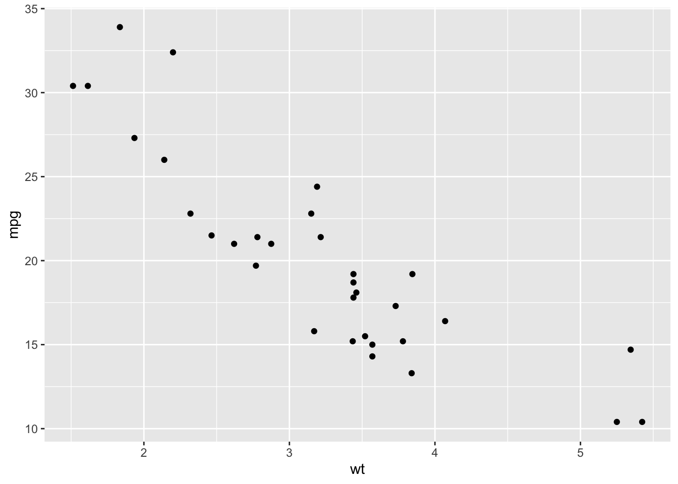
ggsave("plot.pdf")## Saving 7 x 5 in imageNotice that the result of dev.size() and the message we receive when saving the plot with ggsave() give the same dimensions.
One strategy we could take to size our plots is to adjust the Plots pane. This allows for us to see how the image will look before we save it. However, this option is not reproducible since it leaves no enduring record.
Instead, a better strategy is to specify the dimensions when we save the image. It usually takes a little back-and-forth between selecting dimensions, saving the file, checking the appearance of the saved file, and adjusting the dimensions and geom sizes.
By default, units are specified in inches, but this can be changed.
ggsave("plot.pdf", width = 6, height = 4)
ggsave("plot.pdf", width = 15, height = 10, units = "cm")
ggsave("plot.pdf", width = 150, height = 100, units = "mm")Geom sizes are specified in millimeters, so saving different plot sizes without adjusting geom sizes can have unintended results where everything is too close or too far apart.
ggsave("too-small.png", width = 1.5, height = 1)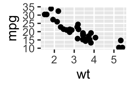
ggsave("too-large.png", width = 12, height = 8)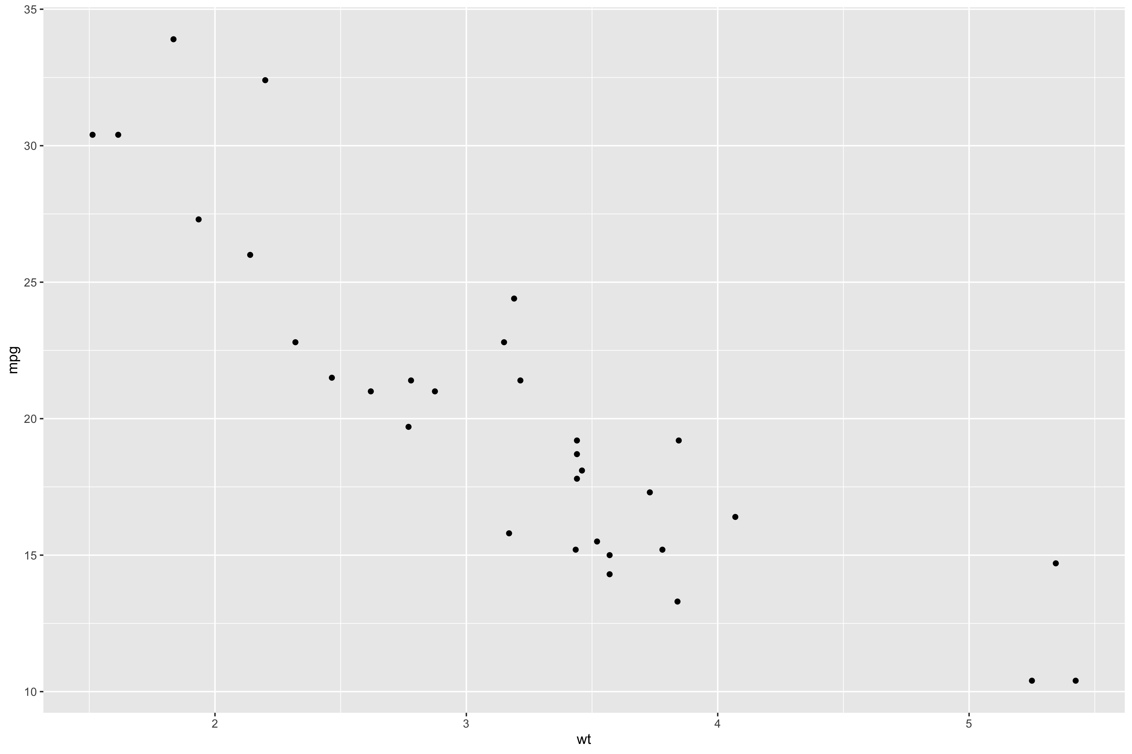
When saving PNGs or other non-vectorized image types (see File Extensions below), the resolution can be specified with dpi, dots (printed pixels) per inch. dpi can be specified as a number, but it also accepts “retina” (320 dpi), “print” (300 dpi), and “screen” (72 dpi).
ggsave("plot.png", dpi = 300)
ggsave("plot.png", dpi = "print")2.1.2 File Names
As with anything else in R, we should give our saved plots different names. If we already have a “plot.pdf” in our working directory, and we save a new “plot.pdf”, it will replace the existing file without any warning.
2.1.3 File Extensions
ggsave() supports several file extensions, which can be found in the table below or with help(ggsave).
| Extension | Vectorized | alpha support | Windows | Linux | macOS |
|---|---|---|---|---|---|
| .bmp | No | Yes | Yes | Yes* | Yes |
| .emf | Yes | Yes | with devEMF | with devEMF | with devEMF |
| .eps | Yes | No | Yes | Yes | Yes |
| .jpeg | No | Yes | Yes | Yes* | Yes |
| Yes | Yes | Yes | Yes | Yes | |
| .png | No | Yes | Yes | Yes* | Yes |
| .ps | Yes | No | Yes | Yes | Yes |
| .svg | Yes | Yes | with svglite | with svglite | with svglite |
| .tex | Yes | Yes | Yes | Yes | Yes |
| .tiff | No | Yes | Yes | Yes* | Yes |
| .wmf | Partial | No | Yes | No | No |
* Must specify type = “cairo”
|
The SSCC Linux servers can be accessed and used in three ways (click each for details): interactively at the command line, in batch mode at the command line, or with an RStudio interface via RStudio Server. When saving plots with extensions .bmp, .jpeg, .png, or .tiff, we must specify type = "cairo" like so: ggsave("plot.png", type = "cairo"). When using the Linux command line options, we need to use cairo in order to save plots with semi-transparency (see Alpha Support). When using RStudio Server, cairo is needed to save these plot types at all.
The file extension can be specified either in the name ("plot.pdf") or in the device argument with quotes (device = "pdf"), or in both places.
However, to save EMF files, we need to first install and load the devEMF package. Then, the file extension needs to be specified in the device argument through a function, and optionally in the file name. See examples below.
ggsave("plot1.pdf")
ggsave("plot1", device = "pdf")
ggsave("plot1.pdf", device = "pdf")
library(devEMF)
ggsave("plot2", device = {function(filename, ...) devEMF::emf(file = filename, ...)})
ggsave("plot2.emf", device = {function(filename, ...) devEMF::emf(file = filename, ...)})EMF and PDF files excel in quality and compatibility with other applications, making them the preferred file types. However, some situations require other file extensions to be used. If that is the case, it is important to know about image vectorization and alpha.
2.1.3.1 Vector Graphics
Images that are vectorized contain instructions for how an image is to be drawn: draw a black line from point A to point B, write the number “10” at point C, and so on.
Images that are not vectorized are coded as tables of color values: the pixel in picture[1, 1] is “white” (represented by some numeric value), picture[1, 2] is “black”, picture[1, 3] is “dark blue”, and so on. Non-vectorized images are also called rasterized or bitmap images.
Because of this difference, vectorized images can be rescaled without any effect on image quality. On the other hand, when if we make a non-vectorized image too large, we might be able to see individual pixels (i.e., pixelization).
To see this, we can save the following plot in a vectorized format (PDF) and a non-vectorized format (PNG).
ggplot(mtcars, aes(x = wt, y = mpg)) +
geom_point() +
geom_abline(intercept = 10, slope = 3, color = "red") +
geom_smooth(se = F)## `geom_smooth()` using method = 'loess' and formula 'y ~ x'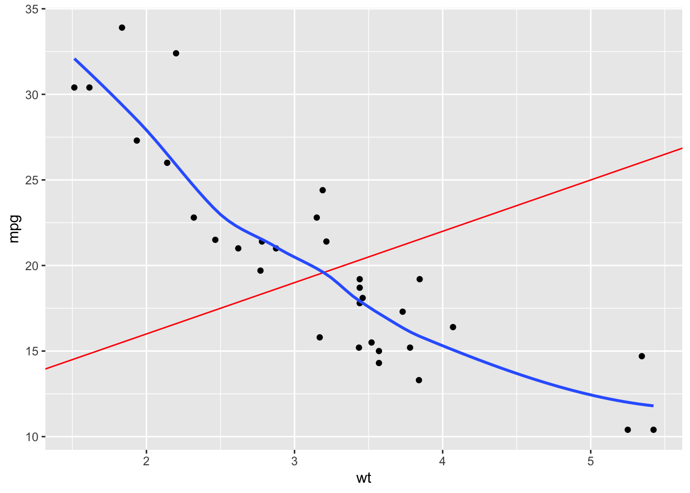
ggsave("plot.pdf")
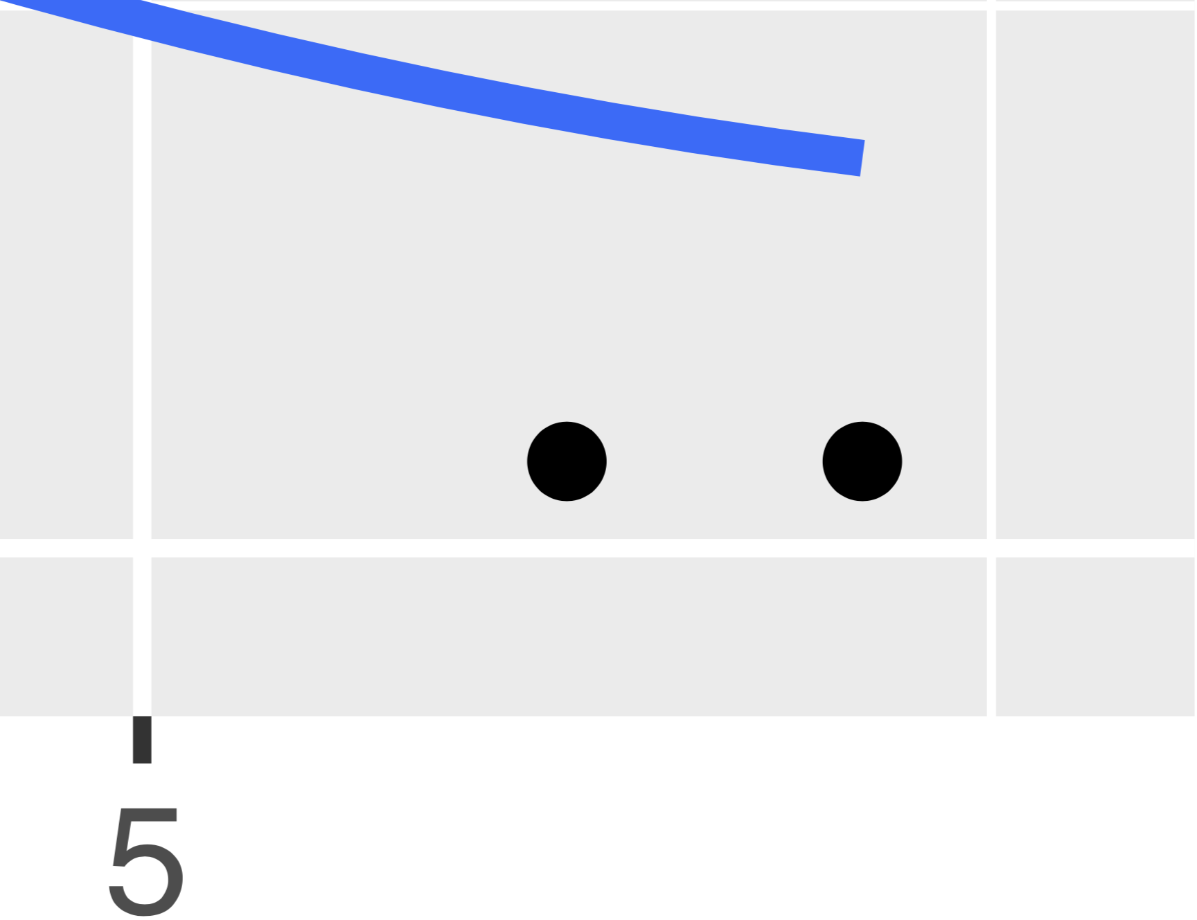
ggsave("plot.png")Compare the image quality if we zoom into the “10” on the y-axis of the two plots:
PDF:
PNG:
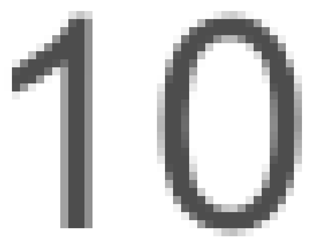
At this level, we can see the individual pixels of the PNG image, while the PDF image retains its quality.
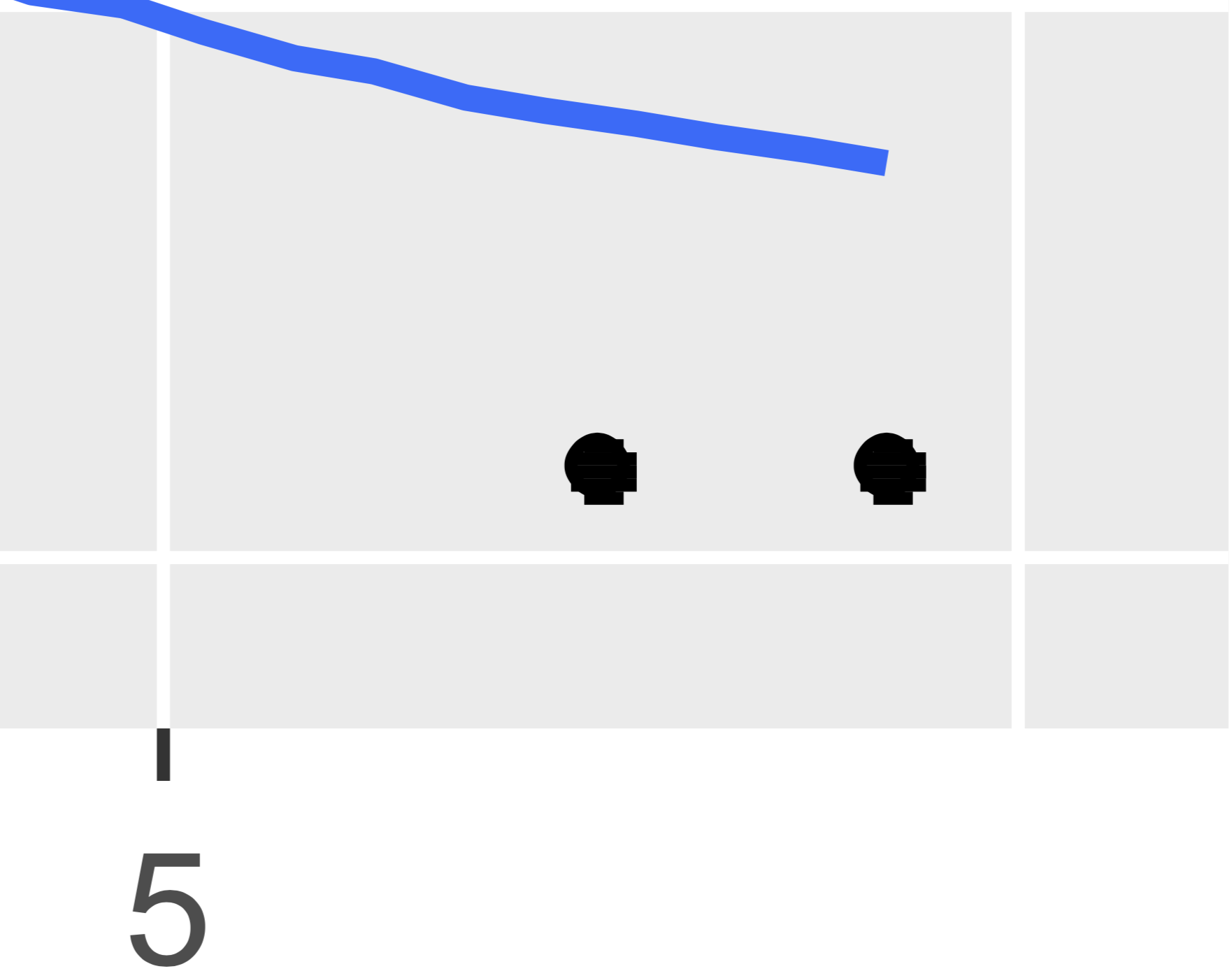
WMF images are only partially vectorized. To see this, we can save our plot with the WMF and EMF extensions.
ggsave("plot.wmf")
ggsave("plot.emf", device = {function(filename, ...) devEMF::emf(file = filename, ...)})
Comparing the two images, the axis labels are vectorized in WMF images, but the geom_smooth() line is slightly more jagged. Additionally, it appears as though WMF plotted two sets of overlapping points, one vectorized (round edges), and another not vectorized (square edges). The EMF image, however, retains its quality and smoothness even when enlarged to this degree.
WMF:
EMF:
Because of this, it is not recommended to save plots with the WMF extension, but the EMF remains as a good option for vectorized images.
Understanding how images are encoded is important when presenting large plots, such as on posters or in presentations. Using a vectorized image format is a good way to ensure your plots retain their quality when enlarged.
2.1.3.2 Alpha Support
The alpha parameter controls the degree of transparency.
Many geoms can be set to be partially transparent with the alpha argument, and geom_smooth() contains a semi-transparent standard error ribbon by default. alpha can range from 0 to 1, where 0 is transparent and 1 is opaque.
The alpha = rep(c(.5, 1), 16) argument makes it so that the alpha level of our first point is 0.5 (half transparent), the second 1 (opaque), the third 0.5, and so on, for all 32 rows in mtcars.
ggplot(mtcars, aes(x = wt, y = mpg)) +
  geom_point(alpha = rep(c(.5, 1), 16)) +
  geom_smooth()
## `geom_smooth()` using method = 'loess' and formula 'y ~ x'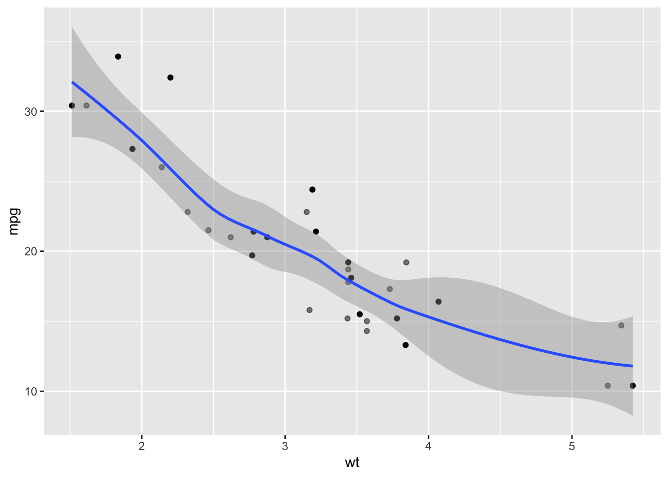
File extensions without alpha support, such as EPS, will simply omit features that are not fully opaque.
ggsave("plot.eps")## Saving 7 x 5 in image## `geom_smooth()` using method = 'loess' and formula 'y ~ x'## Warning in grid.Call.graphics(C_points, x$x, x$y, x$pch, x$size): semi-
## transparency is not supported on this device: reported only once per page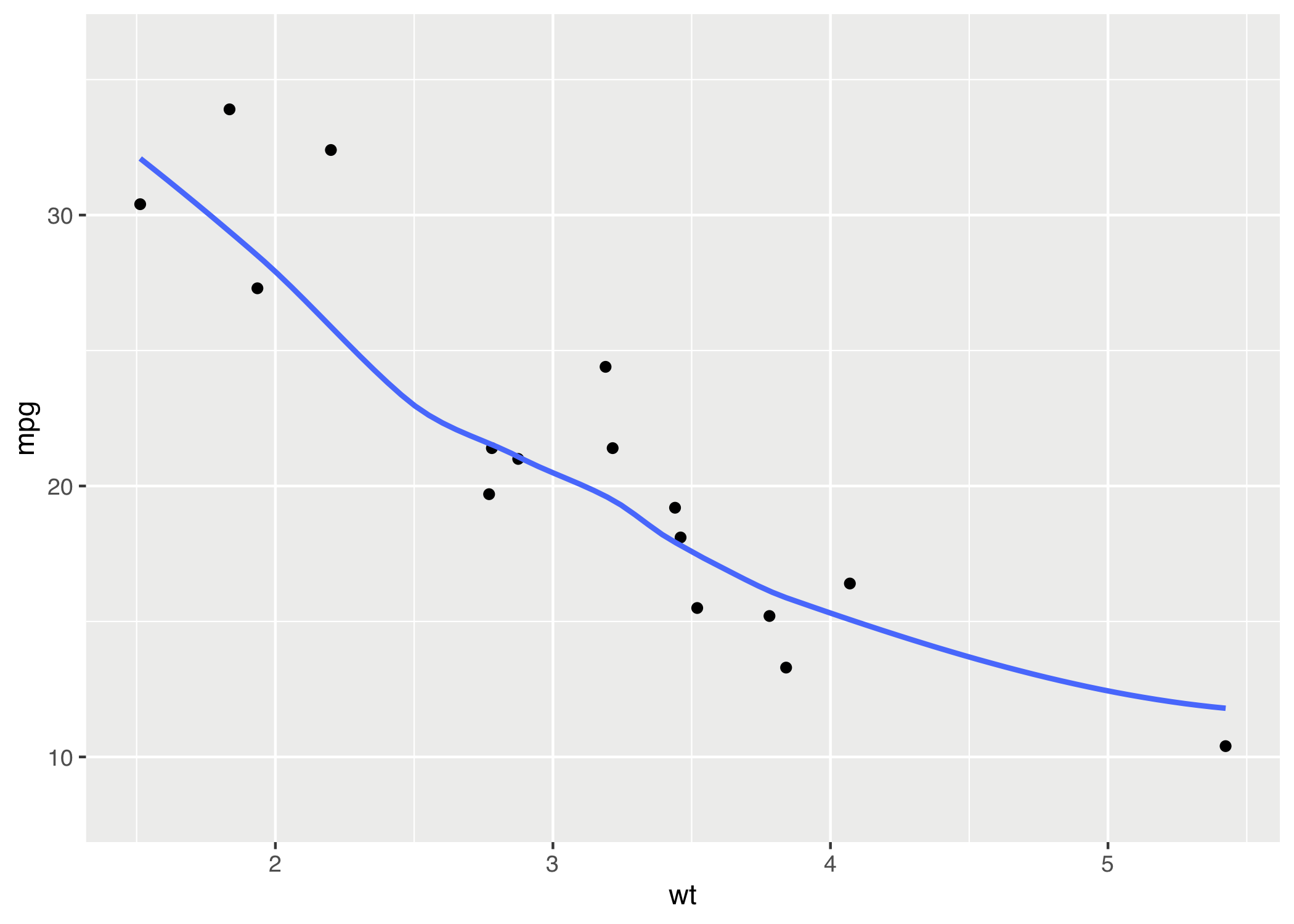
Notice that the half-transparent points and the light gray standard error ribbon from geom_smooth() are not shown in the plot.
2.2 Other Options for Saving Plots
2.2.1 Graphics Devices (Base R Plots)
If we create plots outside of ggplot (with plot(), hist(), boxplot(), etc.), we cannot use ggsave() to save our plots since it only supports plots made with ggplot.
Base R provides a way to save these plots with its graphic device functions. Instead of a two step process of (1) creating a plot and then (2) saving it as with ggsave(), we have three steps when using base R:
- Specify the file extension and properties (size, resolution, etc.) .
- Supported extensions:
bmp(),jpeg(),png(),tiff(),pdf(), andemf()(load thedevEMFpackage first) - Units can be specified in pixels (
px, the default for the first four extensions), inches (in, the default forpdf()andemf()), centimeters (cm), or millimeters (mm).
- Create the plot with base R, ggplot, or any other plotting package.
- Note: After opening the graphics device in step 1, the plot will not be shown in the Plots pane
- Signal that the plot is finished and save it by running
dev.off().
Here are three examples, one made with ggplot() and saved as a PNG, and two made with base R’s plot() and saved as a PDF and as an EMF.
png(filename = "plot3.png", width = 6, height = 4, units = "in", res = 300)
ggplot(mtcars, aes(x = wt, y = mpg)) +
  geom_point() +
  geom_abline(intercept = 10, slope = 3, color = "red")
dev.off()

pdf(file = "plot4.pdf", width = 6, height = 4)
plot(mtcars$wt, mtcars$mpg)
abline(a = 10, b = 3, col = "red")
dev.off()

emf(file = "plot5.emf", width = 6, height = 4)
plot(mtcars$wt, mtcars$mpg)
abline(a = 10, b = 3, col = "red")
dev.off()
2.2.2 RStudio Interface
RStudio provides a point-and-click method to save plots in the Plots pane. This method is not recommended, however, because it leaves no record and is thus not reproducible.
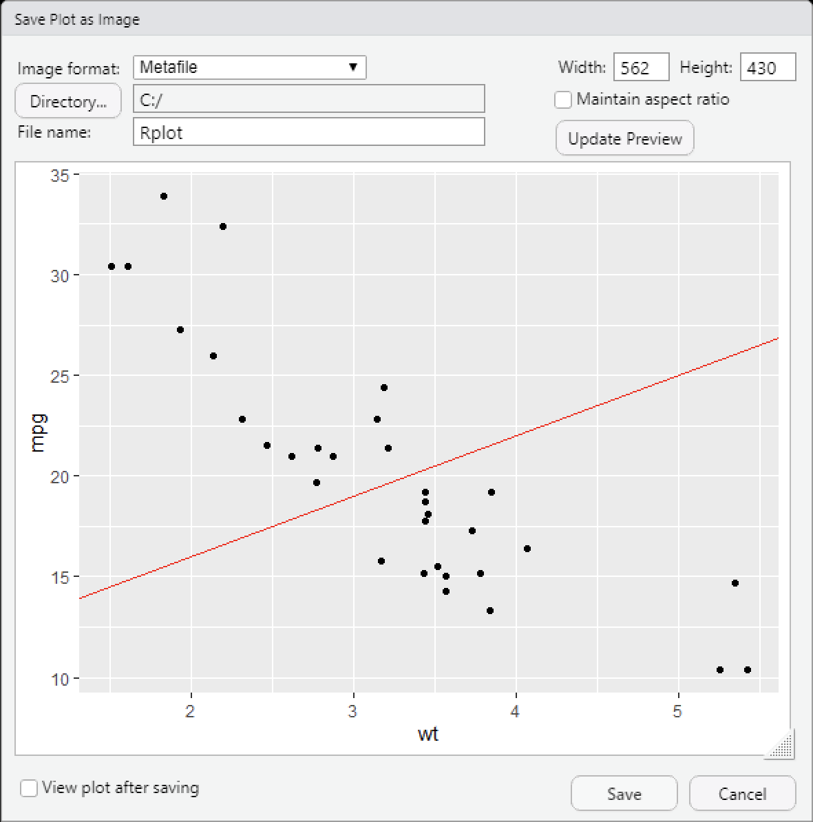
To save a plot in this way, first create the plot, and then click on Export in the Plots pane.
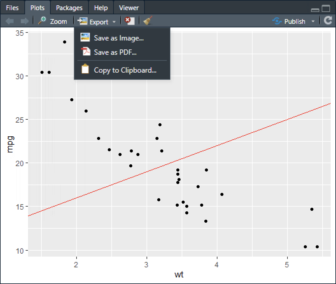
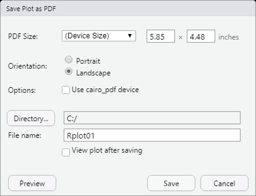
Selecting Save as Image… yields the dialog below. Several image formats are supported: PNG, JPEG, TIFF, BMP, EMF (here called “Metafile”), SVG, and EPS. The plot dimensions (in pixels), path, and name can be chosen here.
In the Export menu, selecting Save as PDF… brings up the menu below, where the plot dimensions (in inches), path, and name can be specified.