9 Categorical
We can divide data into two general categories: continuous and categorical. Continuous data is numeric, has a natural order, and can potentially take on an infinite number of values. Examples include age, income, and health care expenditures. In contrast, categorical data takes on a limited number of values and may or may not have a natural order. Examples without a natural order include race, state of residence, and political affiliation. Examples with a natural order include Likert scale items (e.g., disagree, neutral, agree), socioeconomic status, and educational attainment.
The distinction between continuous and categorical variables is fundamental to how we use them the analysis. For example, in a regression model, continuous variables give us slopes while categorical variables give us intercepts.
In R, categorical data is managed as factors. We specify which variables are factors when we create and store them, and then they are treated as categorical variables in a model without any additional specification. This contrasts with other software like Stata, SAS, and SPSS, where we specify which variables are categorical in our model syntax.
9.1 Factor Structure
Understanding how R represents factors will help us understand how to manipulate them.
Let’s begin with a simple character vector, x, that contains the letters a, b, c, and d.
x <- c("a", "b", "c", "b", "d", "a", "a")When we print x, R quotes the values:
x[1] "a" "b" "c" "b" "d" "a" "a"Now, make a factor called y from x with the factor() function. y prints differently than x. It does not have quotes around its values, and it contains a line about something called “levels,” which contains the unique values of y.
y <- factor(x)
y
[1] a b c b d a a
Levels: a b c dA factor is composed of two parts: an integer vector and an ordered label vector. To see the underlying integer vector of y, we can coerce it to numeric with as.numeric():
as.numeric(y)[1] 1 2 3 2 4 1 1And we can see the ordered labels with the levels() function:
levels(y)[1] "a" "b" "c" "d"The label “a” is the first level, “b” the second, “c” the third, and “d” the fourth. Factor levels are ordered alphabetically by default. We could make a key as follows:
| Integer | Label |
|---|---|
| 1 | a |
| 2 | b |
| 3 | c |
| 4 | d |
Now, our y factor is actually an integer vector, but when we print it, R shows the corresponding labels.
Compare the output from y and as.numeric(y) once again, and refer to the table above.
y
[1] a b c b d a a
Levels: a b c d
as.numeric(y)
[1] 1 2 3 2 4 1 19.2 Factor Defaults
When we include a character variable when plotting or modeling in R, R treats it as a factor, and its default is to
- sort levels alphabetically by their label
- leave the existing labels as-is
- include all unique values
Why are these problems?
To see why this is not ideal, let’s create some survey response data, where individuals could indicate whether they agreed, neither agreed nor disagreed, or disagreed with a statement, or if the statement did not apply to them (“not applicable”). Individuals could also choose to not answer the question (“no answer”).
answers <- c("AGREE",
             "NEITHER",
             "DISAGREE",
             "NOT APPLICABLE",
             "NO ANSWER")
responses <- sample(answers, 100, replace = T)
Now, make a plot of counts by response.
library(ggplot2)
ggplot() + geom_bar(aes(responses))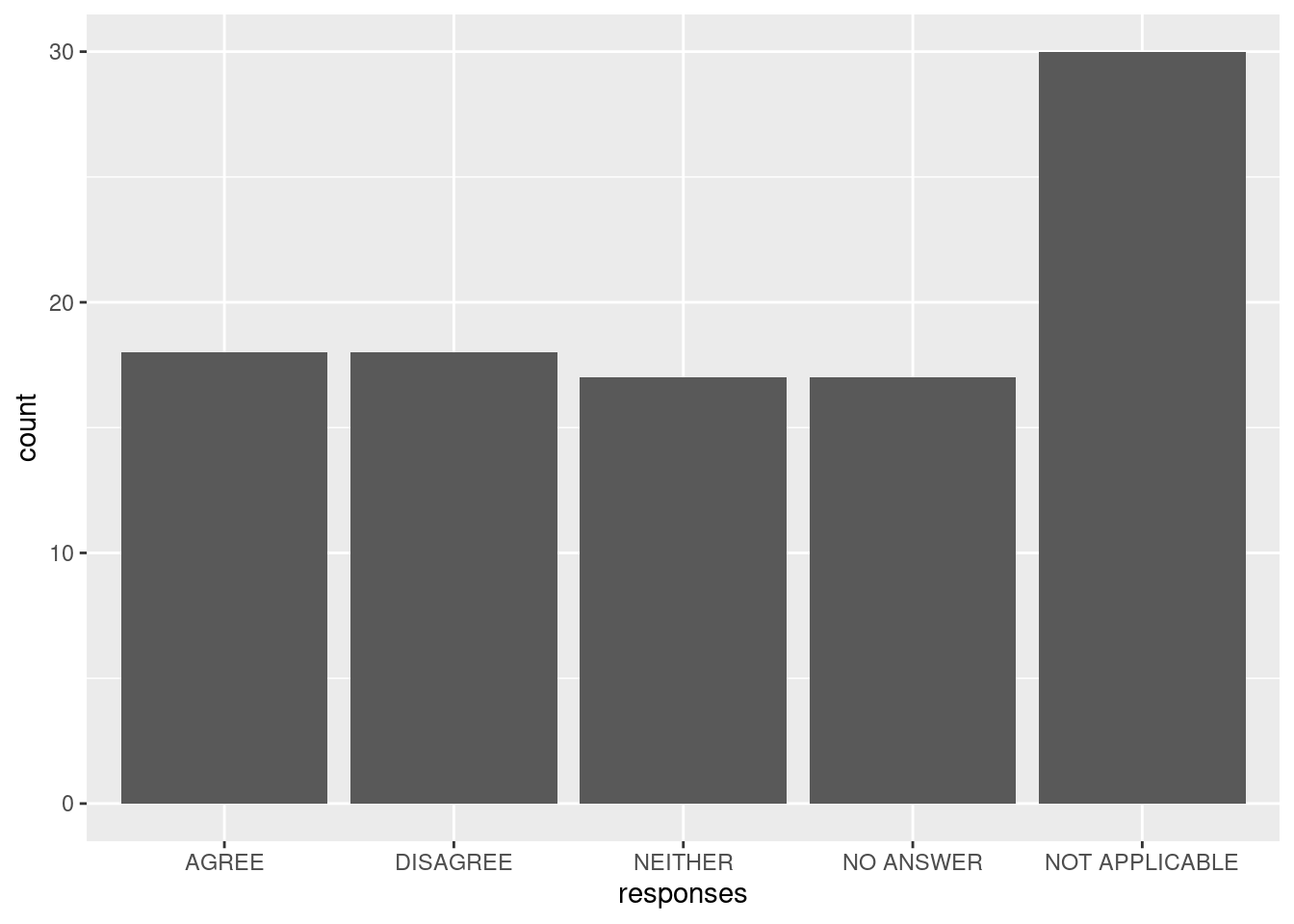
(See more on using ggplot2 in Data Visualization in R with ggplot2.)
We can see R’s defaults in action:
- The variable was ordered alphabetically, but it would make more sense to have “neither” between “agree” and “disagree.”
- The labels were used as-is, but we might choose to not use all-uppercase labels to improve the appearance of the plot (i.e., “Agree” rather than “AGREE”).
- All values in our data were included, but we might consider combining the two categories of “no answer” and “not applicable” to a single “missing.”
We will learn how to manipulate these three aspects of factors in R: order (releveling), labels (recoding), and number of categories (collapsing). For all of these operations, we will be making use of the forcats library, which makes it easy to manipulate factors.
9.3 Releveling
When we relevel a factor, we change the order of its levels. If we give fct_relevel() the name of a factor and the name of a level, it moves that level to the first position and leaves the others in their current order.
First, load the forcats library.
library(forcats)Using y from earlier, create y_relevel, which has “b” instead of “a” as its first level.
y_relevel <- fct_relevel(y, "b")The levels of y_relevel are as follows:
| Integer | Label |
|---|---|
| 1 | b |
| 2 | a |
| 3 | c |
| 4 | d |
Compare the output from y and y_relevel when printing them as is, printing their underlying integers, and printing their levels.
y
[1] a b c b d a a
Levels: a b c d
y_relevel
[1] a b c b d a a
Levels: b a c d
as.numeric(y)
[1] 1 2 3 2 4 1 1
as.numeric(y_relevel)
[1] 2 1 3 1 4 2 2
levels(y)
[1] "a" "b" "c" "d"
levels(y_relevel)
[1] "b" "a" "c" "d"
The data still prints the same, but the order of the levels has changed, and this is reflected in the integer output. In y_relevel, “b” is 1 and “a” is 2.
9.3.1 Changing the Reference Level
We can use R’s built-in chickwts dataset, which has a factor variable called feed.
str(chickwts)'data.frame': 71 obs. of 2 variables:
$ weight: num 179 160 136 227 217 168 108 124 143 140 ...
$ feed : Factor w/ 6 levels "casein","horsebean",..: 2 2 2 2 2 2 2 2 2 2 ...The first, or reference, level of feed is “casein”:
levels(chickwts$feed)[1] "casein" "horsebean" "linseed" "meatmeal" "soybean" "sunflower"If we make box plots of weight by feed, we see that “casein” is the first variable on the x-axis:
plot(weight ~ feed, chickwts)
And if we predict weight by feed in a linear model, we will get this output:
lm(weight ~ feed, chickwts)
Call:
lm(formula = weight ~ feed, data = chickwts)

Coefficients:
  (Intercept)  feedhorsebean    feedlinseed   feedmeatmeal    feedsoybean  feedsunflower
      323.583       -163.383       -104.833        -46.674        -77.155          5.333
Our reference level, casein, is omitted since it is represented by the intercept. The other feeds’ coefficients are comparisons to the reference category, or adjustments to the intercept. In R model output, the coefficients for the levels of a factor variable are labeled with the variable name followed by the level label, so the coefficient for the horsebean level of the feed variable is called feedhorsebean.
If we want to change the ordering of a categorical variable in a plot or change the reference level in a statistical model, we should relevel our factor. We can make another variable in chickwts called feed2 where “soybean” is the reference level:
chickwts$feed2 <- fct_relevel(chickwts$feed, "soybean")Now, if we plot weight by feed with feed2, “soybean” is the first value on the x-axis, followed by “casein” and all the other levels.
plot(weight ~ feed2, chickwts)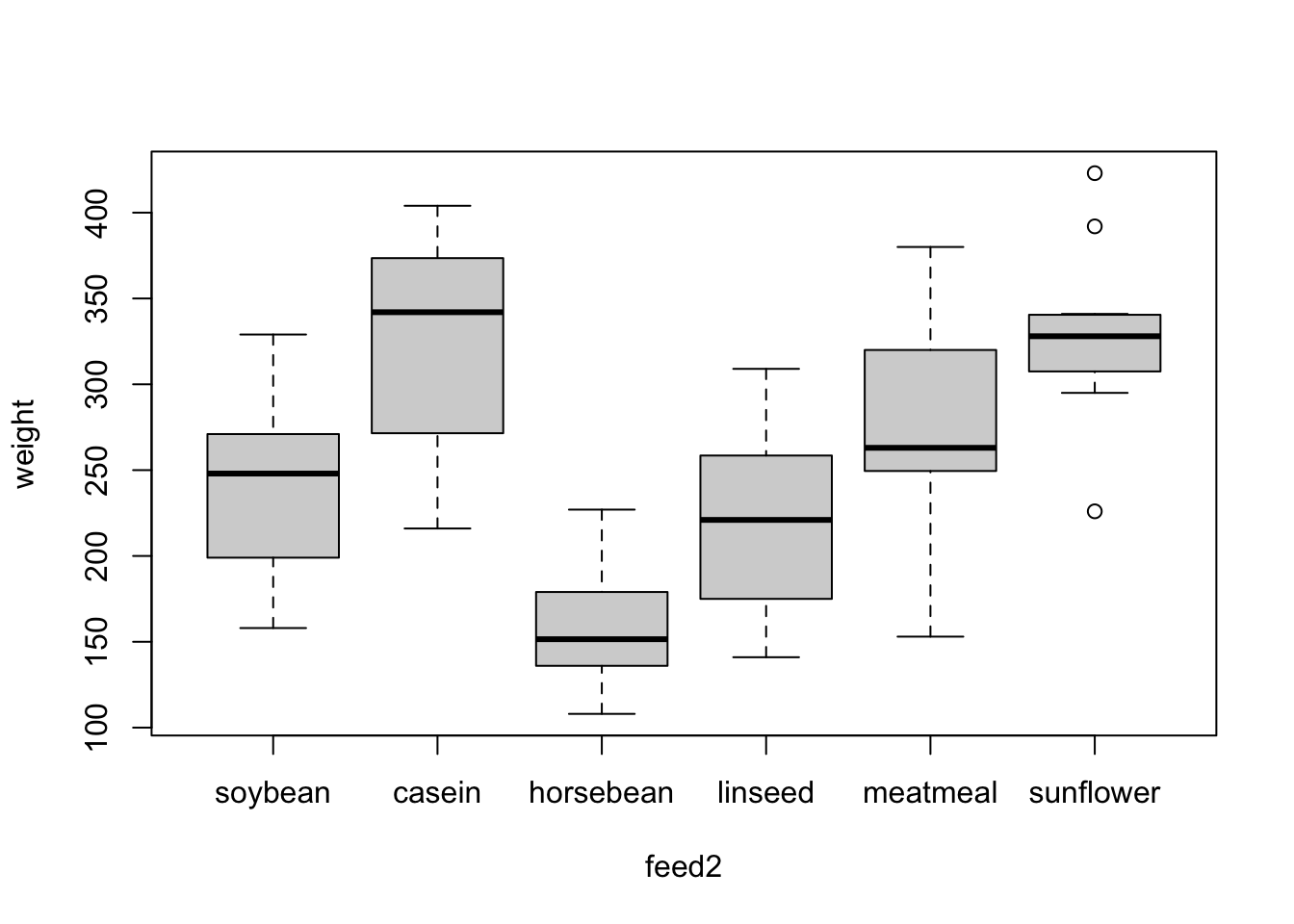
And if we fit our model again with feed2, we see that the intercept has changed since it now represents the expected value of weight when the feed is set to “soybean.” If we want to calculate the expected value for casein, we would add its coefficient (77) to the intercept (246), resulting in an estimate of 323. This matches the intercept in our previous model!
lm(weight ~ feed2, chickwts)
Call:
lm(formula = weight ~ feed2, data = chickwts)

Coefficients:
   (Intercept)     feed2casein  feed2horsebean    feed2linseed   feed2meatmeal  feed2sunflower
        246.43           77.15          -86.23          -27.68           30.48           82.49
9.3.2 Changing All the Levels
So far we have only specified one level with fct_relevel(), but we can specify as many levels as we want, up to the number of levels in our factor. Anything we do not name will follow those we do name.
This is useful when our factor levels have a natural order, like responses on a Likert scale:
survey <- c("Strongly agree",
            "Agree",
            "Neither agree nor disagree",
            "Disagree",
            "Strongly disagree")
survey <- factor(survey)
levels(survey)
[1] "Agree"                      "Disagree"                   "Neither agree nor disagree" "Strongly agree"
[5] "Strongly disagree"
survey <- fct_relevel(survey,
                      "Strongly agree",
                      "Agree",
                      "Neither agree nor disagree",
                      "Disagree",
                      "Strongly disagree")
levels(survey)
[1] "Strongly agree"             "Agree"                      "Neither agree nor disagree" "Disagree"
[5] "Strongly disagree"
9.4 Recoding
Recoding is changing the labels on our factors. To do this, we can supply fct_recode() with our factor and a series of new_label = current_label pairs. Anything we do not name will be left in its existing state.
Using y again, create y_recode, which has full fruit names instead of just their first letters:
y_recode <- fct_recode(y,
                       "apple" = "a",
                       "banana" = "b",
                       "cantaloupe" = "c",
                       "durian" = "d")
The levels of y_recode are as follows:
| Integer | Label |
|---|---|
| 1 | apple |
| 2 | banana |
| 3 | cantaloupe |
| 4 | durian |
Only the labels of the data are changed when recoding. The order and the underlying numeric values remain the same.
y
[1] a b c b d a a
Levels: a b c d
y_recode
[1] apple      banana     cantaloupe banana     durian     apple      apple
Levels: apple banana cantaloupe durian
as.numeric(y)
[1] 1 2 3 2 4 1 1
as.numeric(y_recode)
[1] 1 2 3 2 4 1 1
levels(y)
[1] "a" "b" "c" "d"
levels(y_recode)
[1] "apple"      "banana"     "cantaloupe" "durian"
With chickwts, we can change how one or more levels are labeled. Perhaps two of the feeds were produced by two companies (A and B), and we can indicate that by changing the labels:
chickwts$feed3 <- fct_recode(chickwts$feed,
                             "Company A" = "soybean",
                             "Company B" = "meatmeal")
levels(chickwts$feed)
[1] "casein"    "horsebean" "linseed"   "meatmeal"  "soybean"   "sunflower"
levels(chickwts$feed3)
[1] "casein"    "horsebean" "linseed"   "Company B" "Company A" "sunflower"
Use the table() function after recoding to verify that the recoding worked as intended:
table(chickwts$feed, chickwts$feed3)
            casein horsebean linseed Company B Company A sunflower
  casein        12         0       0         0         0         0
  horsebean      0        10       0         0         0         0
  linseed        0         0      12         0         0         0
  meatmeal       0         0       0        11         0         0
  soybean        0         0       0         0        14         0
  sunflower      0         0       0         0         0        12
The first argument of table() (feed) is the rows, and the second (feed3) is the columns. We can see that wherever we had “meatmeal” or “soybean” in feed, we have “Company B” or “Company A” in feed3, respectively.
9.4.1 Make Levels Missing
Missing values can be coded in a variety of ways. To turn a level of a factor into missing, recode it as NULL.
All the corresponding values are converted to NA, and the level we made missing is removed from the levels() output.
y_miss <- fct_recode(y, NULL = "b")
y_miss
[1] a    <NA> c    <NA> d    a    a
Levels: a c d
as.numeric(y_miss)
[1]  1 NA  2 NA  3  1  1
levels(y_miss)
[1] "a" "c" "d"
9.4.2 Numeric Categorical Variables
Sometimes, variables appear to be continuous, numeric variables, but they are actually categorical variables.
An example of this is if we have Likert scale data. Responses may range 1-5 and represent level of agreement. Some may argue that we can treat such a variable as continuous, but for now we will force it to be categorical.
survey <- sample(1:5, 100, replace = T)If we were to pass survey to fct_recode(), we will get an error:
survey <- fct_recode(survey,
                     "Strongly agree" = 1,
                     "Agree" = 2,
                     "Neither agree nor disagree" = 3,
                     "Disagree" = 4,
                     "Strongly disagree" = 5)
Error in `fct_recode()`:
! `.f` must be a factor or character vector, not an integer vector.This is because fct_recode() (as well as all the other fct_*() functions) require a character or factor vector. If we want to manipulate a numeric vector, first coerce it to a character, and then recode it. We need to be sure to quote the right half of each of our recoding pairs, since survey’s values are now character (e.g., "1") rather than numeric (1).
survey <- fct_recode(as.character(survey),
                     "Strongly agree" = "1",
                     "Agree" = "2",
                     "Neither agree nor disagree" = "3",
                     "Disagree" = "4",
                     "Strongly disagree" = "5")
9.5 Collapsing
Another factor manipulation is reducing the number of levels, called collapsing. Sometimes we have a factor with many levels, but very few observations exist at some levels. This can cause problems in estimation, especially in logistic regression models. We can combine levels with few observations together.
We can do this with fct_collapse(), and our arguments follow the pattern new_level = c(current_level_1, current_level_2, ...).
We can combine levels from y so that “a” is in a new level called “vowel”, and the other three letters (“b”, “c”, and “d”) are combined into a group called “consonant.”
y_collapse <- fct_collapse(y,
                           "vowel" = "a",
                           "consonant" = c("b", "c", "d"))
Our levels for y_collapse are now as follows:
| Integer | Label |
|---|---|
| 1 | vowel |
| 2 | consonant |
This process is irreversible since we have lost data. We could change “vowel” back into “a” with fct_recode() since this level of y_collapse is only composed of one level from y. However, because “consonant” is a composite of multiple levels, it is impossible to separate this level back into “b”, “c”, and “d”. Therefore, it is a good idea to create a new object or variable when collapsing a factor.
Compare the output and structure of y and y_collapse to see how the data has changed:
y
[1] a b c b d a a
Levels: a b c d
y_collapse
[1] vowel     consonant consonant consonant consonant vowel     vowel
Levels: vowel consonant
as.numeric(y)
[1] 1 2 3 2 4 1 1
as.numeric(y_collapse)
[1] 1 2 2 2 2 1 1
levels(y)
[1] "a" "b" "c" "d"
levels(y_collapse)
[1] "vowel"     "consonant"
After collapsing, we should compare the original and new factors to verify the coding worked as intended:
table(y, y_collapse) y_collapse
y vowel consonant
a 3 0
b 0 2
c 0 1
d 0 1All the values of “a” in y correspond to “vowel” in y_collapse, while “b”, “c”, and “d” correspond to “consonant.”
9.5.1 Empty Levels
If we take a subset of our data, the levels data for factor variables remains unchanged, even if we have excluded all observations at a certain level.
Take a subset of the first five values of chickwts and store them as chickwts_subset.
chickwts_subset <- chickwts[1:5, ]The levels data for chickwts_subset still includes all six types of feed, even though we only have “horsebean” in our subset.
chickwts_subset$feed
[1] horsebean horsebean horsebean horsebean horsebean
Levels: casein horsebean linseed meatmeal soybean sunflower
as.numeric(chickwts_subset$feed)
[1] 2 2 2 2 2
levels(chickwts_subset$feed)
[1] "casein"    "horsebean" "linseed"   "meatmeal"  "soybean"   "sunflower"
This can have some annoying consequences for some plots, where levels with no observations are still included:
plot(weight ~ feed, chickwts_subset)
To remove these extra levels, simply use factor() to “reset” the factor and drop unused levels:
chickwts_subset$feed <- factor(chickwts_subset$feed)Now verify that these levels were removed:
chickwts_subset$feed
[1] horsebean horsebean horsebean horsebean horsebean
Levels: horsebean
as.numeric(chickwts_subset$feed)
[1] 1 1 1 1 1
levels(chickwts_subset$feed)
[1] "horsebean"
plot(weight ~ feed, chickwts_subset)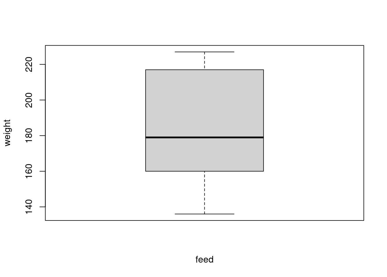
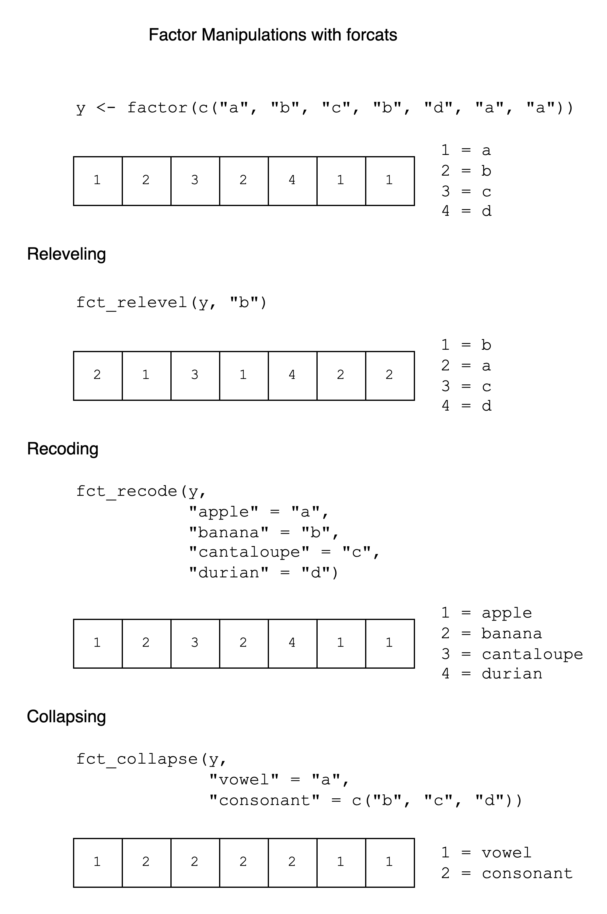
9.6 Cheat Sheet
A simple cheat sheet for factor manipulation is given below. It has examples of fct_relevel(), fct_recode(), and fct_collapse() with the y vector, showing the integer vector and integer-label mapping after each operation.
9.7 Exercises
Releveling: Using the
irisdataset, plot counts by factor level withplot(iris$Species). Now, relevelSpeciesso thatversicoloris the reference (first) category. Plot it again. What do you notice?Recoding: In the
mtcarsdata, all the variables are numeric. Convertvsto a factor, where 0 has the label “V-shaped” and 1 has the label “Straight”.Collapsing:
mtcars$cylhas three different values: 4, 6, and 8. Convert it into a two-level factor, where 4 and 6 share the label “Few” and 8 has the label “Many”.