10 Reading Text Data
The examples on this page require example files, which you can download by clicking on the link below. After downloading, extract the files to a folder.
10.1 Paths and Working Directories
If you need to work on multiple projects simultaneously, use R Projects (capital “P”). This page does not cover R Projects, but they are discussed in R for Data Science and What They Forgot to Teach You About R. In this chapter, we will assume you are only working on one project at a time, and this makes the overhead of R Projects unnecessary.
Working directories are often a foreign concept for individuals who are new to programming or whose introduction to computers has been through graphical desktops, where you point and click to open files and use dialogs to save files.
10.1.1 Working Directories?
Imagine I just opened RStudio and started a script called myScript.R. I then downloaded a file (dataset.csv), which I now want to import into R. I see the file in my Downloads folder, so I tell R to just import it:
dat <- read.csv("dataset.csv")Warning in file(file, "rt"): cannot open file 'dataset.csv': No such file or directoryError in file(file, "rt"): cannot open the connectionUh-oh. I can see the file, but R cannot. Where is R looking? What does it see?
R looked for dataset.csv in its working directory.
ⓘ Working Directory
A working directory is the folder where the software looks for files. It is the default for reading/loading and writing/saving files.
We can ask for the working directory with getwd():
getwd()[1] "/Users/bbadger/Documents/"(We can change our working directory in a few ways, and even set the default on launch in Global Options, but we will learn another trick below.)
In that directory (which we more commonly call a “folder”), what does R see? R can tell us with list.files():
list.files()[1] "myScript.R" "HW1.pdf" Notably, dataset.csv is missing from this list, and this is why R gave us the No such file or directory error when we tried to import it. How can we tell R how to find the file?
10.1.2 Setting the Working Directory
Rstudio has a wonderful functionality that, if we launch RStudio by double-clicking on a script, it will make the folder containing that script our working directory.
We need to do two things to take advantage of this functionality:
Organize files outside of R. See the sections that follow.
Launch R with scripts. First, be sure RStudio is closed. Then, launch RStudio by double-clicking on a script. Your working directory will be set to the location of that script! There is no need to set our working directory manually with
setwd(). We only need to give R directions on where to read or write files relative to the location of the script, called a relative path.
ⓘ Paths
A path is directions for the software on how to find a file or folder. Paths can be relative or absolute. Relative paths start from the working directory, and absolute paths start from the root directory:
- Windows: U:/Documents/myProject/scripts
- Mac: /Users/bbadger/Documents/myProject/scripts or ~/Documents/myProject/scripts
- Linux: /home/b/bbadger/Documents/myProject/scripts or ~/Documents/myProject/scripts
Relative paths are preferred for most situations because they are shorter, portable, and resistant to breaking if upstream folders are renamed.
10.1.3 Paths and Folder Structures
10.1.3.1 Simple Structure: Files in a Folder
When to use this structure: For minor projects or homework assignments where you have only one or two of each kind of file (script, data, output, etc.).
How it is structured: All files are in a single folder.
If we have two files, myScript.R and dataset.csv and place them in a single folder, myProject, we can visualize the structure like this:
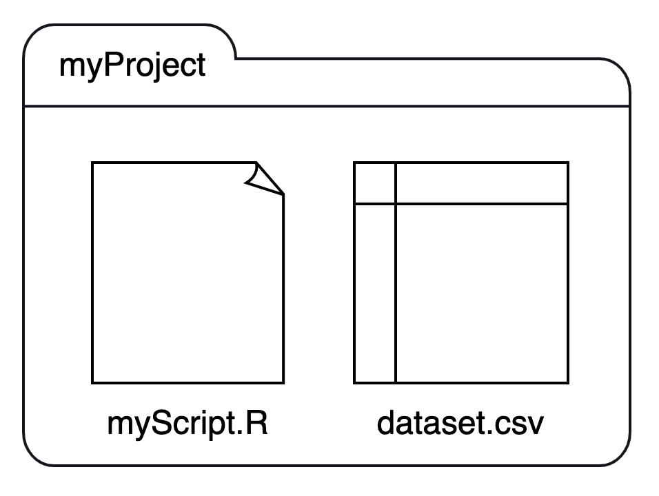
We can recast this structure as a small family tree, where myProject is a parent with two children:

Using this structure: If we launched RStudio by double-clicking on myScript.R, our working directory would be set to myProject. If we want to import dataset.csv, we can run read.csv("dataset.csv") without specifying a path before the file name.
Key idea: If we tell R to read (or write) a file without giving a path name, R will assume it is in the same folder, that it is a sibling of our script.
10.1.3.2 Complex Structure: Files in Folders in a Folder
When to use this structure: For any substantive research, including semester projects, thesis or dissertation research, and collaborative work.
How it is structured: Files are separated into folders by their kinds, with scripts in one folder and data in another. The top-level folder contains a series of folders, and those folders contain files.
Imagine we have a project of medium complexity, where we need to clean, summarize, and model multiple datasets, and produce plots with the results. This project would have started with a single script and a single data file (just like the simple structure above), but after some time, we may have created a new script for each task, downloaded more raw data files, and saved images of plots. Sooner rather than later, we should impose order on our folder structure.
We could separate the files by their types or kinds like this:
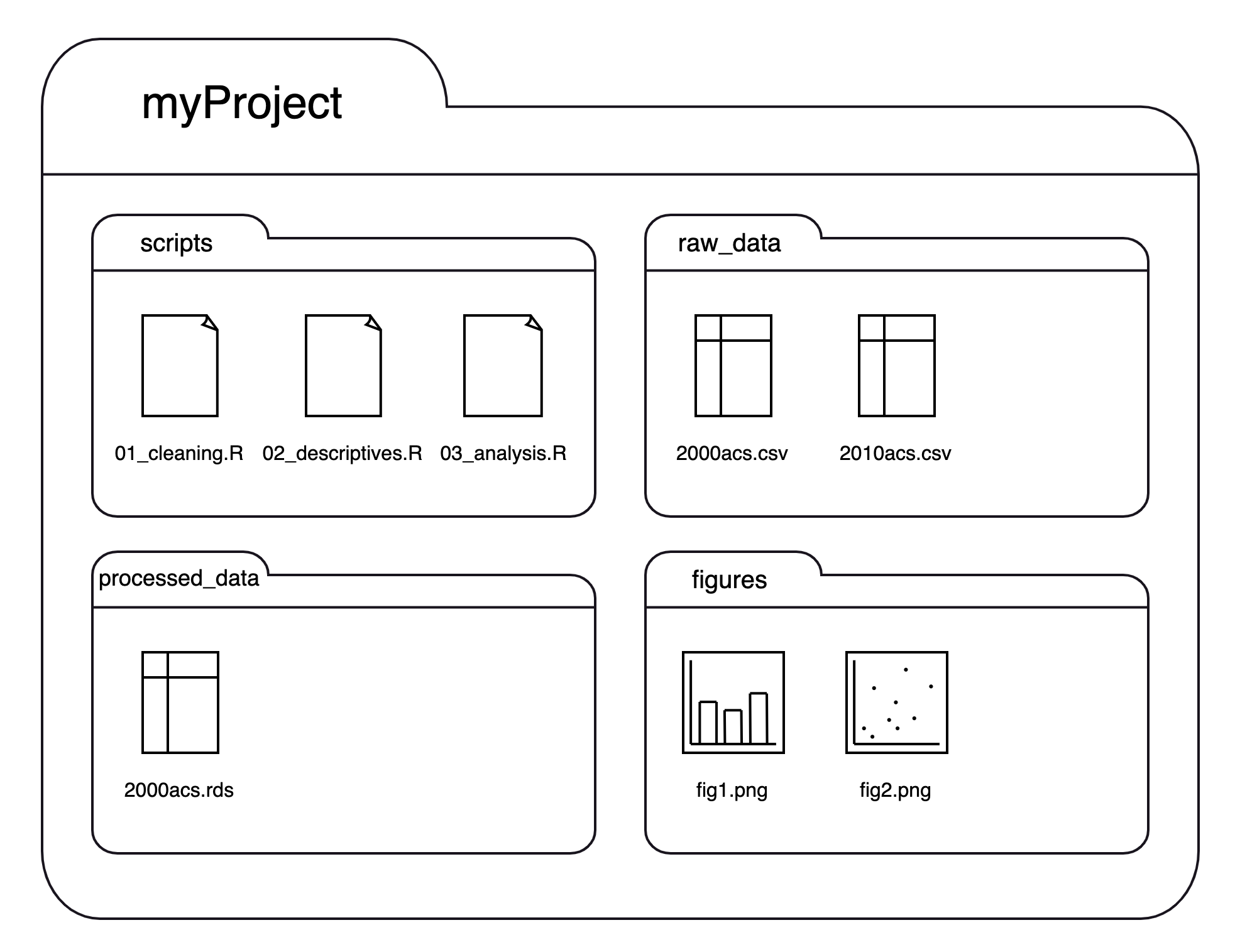
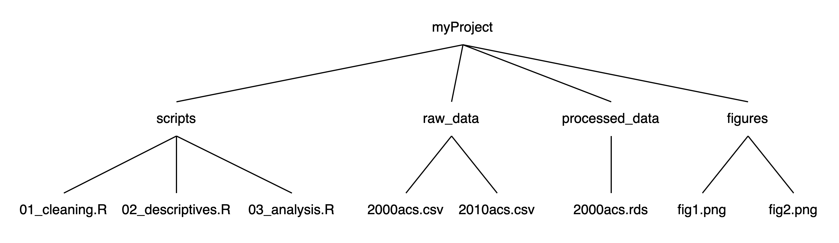
If we think of this structure as a family tree, we now have three generations, where myProject is the grandparent folder who has four children folders, each of which has 1-3 children files of their own:
Using this structure: If we launched RStudio by double-clicking on one of the scripts in the scripts folder, our working directory would be myProject/scripts. To read a script in raw_data, we first need to tell R to (1) get out of our current folder and then (2) go into the raw_data folder. We can move out of folders with .. and into folders with their names. Each step of the path is separated by a slash (/). If we want to import 2000acs.csv, we can run read.csv("../raw_data/2000acs.csv").
Key idea: If we want R to read (or write) a file that is not a sibling of our script, we need to give it a trace of the family relation: .. to move up the family tree, and folder names to move down the tree.
10.1.3.3 More Complex Structures: Files in Folders in Folders … in a Folder
We are not limited to a two-level structure for folders. We can always have more folders within folders, such as if we wanted to create subfolders within the figures folder for descriptives, margins, and diagnostics. The principles from the previous section remain the same: give slash-separated steps of how to find a file: .. to move up and folder names to move down.
To move up two folders, the path would be ../.., and to move down two folders, the path would be folder1/folder2.
If we are in myProject/scripts1/scripts2, and we want to read a CSV in myProject/data1/data2/data3, we would first need to move up two levels into myProject (the first level at which the two paths share a common ancestor), and then down three levels into data3.
To import a file called dataset.csv inside that data3 folder, we would run read.csv("../../data1/data2/data3/dataset.csv")
10.2 Text Data Concepts
A typical project begins by reading data from somewhere into a data frame. A typical data source might be a text file, but it is also possible to import data from binary data files such as those used by Stata, SAS, and SPSS.
Text files come in many forms. It is always a good idea to look at any documentation you have first. Then it can be informative to look at the text file itself, preferably in a dedicated text editor (on SSCC computers, use Notepad++).
You are looking for a few things when you examine the file.
Data, metadata, extra text
The file includes data values. Does it also include variable names or other information that helps define the data? Is there a header or a footer with explanatory text about the file contents?
Observation delimiter
What separates one observation from the next? Commonly, each observation has a separate line in the text file, but it is possible to have multiple observations per line, or multiple lines per observation.
Data value delimiter
Within an observation, what separates one data value from the next? Very commonly the data value delimiter will be a space or a comma. Tabs used to be common, and are hard to distinguish visually from spaces.
Especially in older data sets, it used to be common for data values to appear in specified columns - e.g. state in columns 3-4 and county in columns 5-7 - with no character delimiting data values.
Character value quote
Where data value delimiters are used, how are the same characters included in character data values? For instance, if the data values are separated by spaces, how do you include a space within a data value? The typical answer is, character data values are enclosed in quotes, either double (“) or single (’) quotes.
Missing value string
How are missing values indicated? This might be by having two data value delimiters with no data value between them. Or there might be a special string that denotes missing data, such as NA, -99, or BBBBBBB. There may be more than one missing value indicator as well, such as -98 and -99.
10.3 Reading Data Files
The examples below read six CSV and text files from our website. If you would rather download the files and read them from a local directory, you can download them all by clicking here.
In the examples that follow, these files were placed into a directory called “read” that is in the working directory. Therefore, the paths to the files are read/filename. To follow along, be sure that the read file is in your working directory. To check what R “sees”, run list.files() and verify that the read folder is there. If it is not, see the section Setting the Working Directory above.
10.3.1 CSV Examples
10.3.1.1 The Simple Case
Consider the file class_simple.csv. The first few lines look like this:
Name,Sex,Age,Height,Weight
Alfred,M,14,69,112.5
Alice,F,13,56.5,84
Barbara,F,13,65.3,98
Carol,F,14,62.8,102.5
Henry,M,14,63.5,102.5
In this file,
- The first line has variable names, and the rest is data.
- There is one observation per line.
- Data values are separated by commas.
- There appear to be no character quotes.
- There appear to be no missing values.
Data like this is very easy to read into R with the read.csv() function:
class_simple <- read.csv("read/class_simple.csv")
head(class_simple)
Name Sex Age Height Weight
1 Alfred M 14 69.0 112.5
2 Alice F 13 56.5 84.0
3 Barbara F 13 65.3 98.0
4 Carol F 14 62.8 102.5
5 Henry M 14 63.5 102.5
6 James M 12 57.3 83.0str(class_simple)'data.frame': 19 obs. of 5 variables:
$ Name : chr "Alfred" "Alice" "Barbara" "Carol" ...
$ Sex : chr "M" "F" "F" "F" ...
$ Age : int 14 13 13 14 14 12 12 15 13 12 ...
$ Height: num 69 56.5 65.3 62.8 63.5 57.3 59.8 62.5 62.5 59 ...
$ Weight: num 112 84 98 102 102 ...10.3.1.2 Characters to Factors
Prior to R-4.0, Name and Sex in the previous example would have been turned into factors automatically. This is no longer the default, but remains an option.
class_simple <- read.csv("read/class_simple.csv", as.is = FALSE) # all character vars to factors
str(class_simple)
'data.frame': 19 obs. of 5 variables:
$ Name : Factor w/ 19 levels "Alfred","Alice",..: 1 2 3 4 5 6 7 8 9 10 ...
$ Sex : Factor w/ 2 levels "F","M": 2 1 1 1 2 2 1 1 2 2 ...
$ Age : int 14 13 13 14 14 12 12 15 13 12 ...
$ Height: num 69 56.5 65.3 62.8 63.5 57.3 59.8 62.5 62.5 59 ...
$ Weight: num 112 84 98 102 102 ...To convert specific columns to factors, do the conversion as a separate step later,
or use a named vector of column classes in a colClasses argument.
The vector values are classes to assign, the names are variable names:
cc <- c(Sex = "factor") # a named vector of column classes
class_simple2 <- read.csv("read/class_simple.csv", colClasses = cc)
str(class_simple2)
'data.frame': 19 obs. of 5 variables:
$ Name : chr "Alfred" "Alice" "Barbara" "Carol" ...
$ Sex : Factor w/ 2 levels "F","M": 2 1 1 1 2 2 1 1 2 2 ...
$ Age : int 14 13 13 14 14 12 12 15 13 12 ...
$ Height: num 69 56.5 65.3 62.8 63.5 57.3 59.8 62.5 62.5 59 ...
$ Weight: num 112 84 98 102 102 ...10.3.1.3 No Header
Now consider the file class_noheader.csv. The first few lines look like this:
Alfred,M,14,69,112.5
Alice,F,13,56.5,84
Barbara,F,13,65.3,98
Carol,F,14,62.8,102.5
Henry,M,14,63.5,102.5
James,M,12,57.3,83
The default use of read.csv() takes the first line to be variable
names, resulting in some nonsense names:
class_noheader <- read.csv("read/class_noheader.csv")
str(class_noheader)
'data.frame': 18 obs. of 5 variables:
$ Alfred: chr "Alice" "Barbara" "Carol" "Henry" ...
$ M : chr "F" "F" "F" "M" ...
$ X14 : int 13 13 14 14 12 12 15 13 12 11 ...
$ X69 : num 56.5 65.3 62.8 63.5 57.3 59.8 62.5 62.5 59 51.3 ...
$ X112.5: num 84 98 102 102 83 ...We now need a header=FALSE argument. We can optionally add a
col.names argument, or add names()<- in a separate step, later.
class_noheader <- read.csv("read/class_noheader.csv", header=FALSE)
str(class_noheader) # default names
'data.frame': 19 obs. of 5 variables:
$ V1: chr "Alfred" "Alice" "Barbara" "Carol" ...
$ V2: chr "M" "F" "F" "F" ...
$ V3: int 14 13 13 14 14 12 12 15 13 12 ...
$ V4: num 69 56.5 65.3 62.8 63.5 57.3 59.8 62.5 62.5 59 ...
$ V5: num 112 84 98 102 102 ...class_noheader <- read.csv("read/class_noheader.csv",
header=FALSE,
col.names = c("name", "sex", "age",
"height", "weight"))
str(class_noheader)'data.frame': 19 obs. of 5 variables:
$ name : chr "Alfred" "Alice" "Barbara" "Carol" ...
$ sex : chr "M" "F" "F" "F" ...
$ age : int 14 13 13 14 14 12 12 15 13 12 ...
$ height: num 69 56.5 65.3 62.8 63.5 57.3 59.8 62.5 62.5 59 ...
$ weight: num 112 84 98 102 102 ...10.3.1.4 Quoted Character Values
Quoting character values is seldom a problem … but sometimes it is. So consider the file class_quotes.csv. The first few lines look like this:
"Name","Sex","Age","Height","Weight"
"B, Alfred","M",14,69,112.5
"Y, Alice","F",13,56.5,84
"M, Barbara","F",13,65.3,98
"P, Carol","F",14,62.8,102.5
"A, Henry","M",14,63.5,102.5
This is what we’d like to see. There are commas within the data values
for Name, but these are all in quotes. The default use of read.csv()
assumes that double quotes or single
quotes delimit character values. If some other character is used, we have
the quote argument we can use. If nothing is used, we could be in trouble!
(We might need a new strategy.)
class_quotes <- read.csv("read/class_quotes.csv")
str(class_quotes)
'data.frame': 19 obs. of 5 variables:
$ Name : chr "B, Alfred" "Y, Alice" "M, Barbara" "P, Carol" ...
$ Sex : chr "M" "F" "F" "F" ...
$ Age : int 14 13 13 14 14 12 12 15 13 12 ...
$ Height: num 69 56.5 65.3 62.8 63.5 57.3 59.8 62.5 62.5 59 ...
$ Weight: num 112 84 98 102 102 ...10.3.1.5 Missing Values
Next, consider the file class_missing.csv. The first few lines look like this:
Name,Sex,Age,Height,Weight
Alfred,M,14,,112.5
Alice,F,13,56.5,84
Barbara,F,13,65.3,98
Carol,F,14,62.8,102.5
Henry,M,14,63.5,102.5
Here we have a missing value for Height in the first observation (and more later in the data set).
class_missing <- read.csv("read/class_missing.csv")
head(class_missing)
Name Sex Age Height Weight
1 Alfred M 14 NA 112.5
2 Alice F 13 56.5 84.0
3 Barbara F 13 65.3 98.0
4 Carol F 14 62.8 102.5
5 Henry M 14 63.5 102.5
6 James M 12 57.3 83.0Depending on the software used to produce the text file, a missing value
might be denoted by two data delimiters with no text in between, as in
this example. In text files produced by R iteself, missing values
are usually denoted by NA. So by default these are turned into missing
values as well. Other software might use another symbol (periods are common,
and dashes sometimes are used), for which we have the na.strings argument.
10.3.2 Space Delimited
For space delimited data, we use a related function, read.table(). Here
a few of the assumptions (defaults) are different. Now spaces are assumed
to delimit data values where before they were assumed to be part of data
values, and vice versa for commas. Files are assumed to have no headers.
The other major arguments work as before.
The first few lines of class_space.txt look like this:
Warning in readLines("read/class_space.txt"): incomplete final line found on 'read/class_space.txt'Name Sex Age Height Weight
Alfred M 14 69 112.5
Alice F 13 56.5 84
Barbara F 13 65.3 98
Carol F 14 62.8 102.5
Henry M 14 63.5 102.5Here we have a header with variable names, which we need to indicate.
class_space <- read.table("read/class_space.txt", header=TRUE)
str(class_space)
'data.frame': 19 obs. of 5 variables:
$ Name : chr "Alfred" "Alice" "Barbara" "Carol" ...
$ Sex : chr "M" "F" "F" "F" ...
$ Age : int 14 13 13 14 14 12 12 15 13 12 ...
$ Height: num 69 56.5 65.3 62.8 63.5 57.3 59.8 62.5 62.5 59 ...
$ Weight: num 112 84 98 102 102 ...10.3.3 Fixed-Width Text
Data in fixed columns is easy to recognize when the data values run together. Even if they do not, this can be a solution when spaces or commas are valid data values and there are no character value quotes. Missing values are typically spaces, as well.
The first few lines of class_fixed.txt look like this:
Warning in readLines("read/class_fixed.txt"): incomplete final line found on 'read/class_fixed.txt'Alfred M1469 112.5
Alice F1356.584
BarbaraF1365.398
Carol F1462.8102.5
Henry M1463.5102.5
James M1257.383Here we need to know how many columns each variable occupies (including spaces). Data documentation is a huge help here.
Notice that the width includes the decimal character.
myWidths <- c(7,1,2,4,5)   # how many columns wide each of the variables is

class_fixed <- read.fwf("read/class_fixed.txt", myWidths)
Warning in readLines(file, n = thisblock): incomplete final line found on 'read/class_fixed.txt'head(class_fixed) V1 V2 V3 V4 V5
1 Alfred M 14 69.0 112.5
2 Alice F 13 56.5 84.0
3 Barbara F 13 65.3 98.0
4 Carol F 14 62.8 102.5
5 Henry M 14 63.5 102.5
6 James M 12 57.3 83.010.3.4 Excel Workbooks
Excel workbooks are another common format for data files. However, any data wrangling we do in Excel, like renaming columns or calculating new ones, is neither recorded nor easily reproducible without re-clicking through menu options (unless we use Visual Basic). So that you have a paper trail of all the work you do with your data, we recommend getting your data into R as early as possible, rather than first cleaning it up in Excel.
Load the readxl library:
library(readxl)The read folder has the one-sheet workbook, class_excel.xlsx. Import it with the read_excel() function:
class_excel <- read_excel("read/class_excel.xlsx")Excel workbooks are often more complicated than your average CSV since they can contain multiple sheets, and a single sheet will often have extra metadata above or below the main dataset, and some sheets even have multiple datasets on a single sheet! The readxl library has functions for all of these situations and will allow you to do things like import specific sheets and cell ranges. Read more in the readxl documentation.
10.3.5 Files from Other Statistical Software
Sometimes you may need to use data from SAS, SPSS, or Stata into R. You may run into this if your colleagues use these programs while you use R, or if you are downloading a public dataset and they only offer one of these formats.
To import the binary data files used by these programs, load the haven library.
library(haven)The read folder has the file class_stata.dta, and the .dta extension tells us it is a Stata file. Use the read_dta() function to import it:
class_stata <- read_dta("read/class_stata.dta")Files from other programs may contain data that R dataframes typically do not have, such as value and variable labels. The haven package has functions for working with these types of metadata. Read more in the haven documentation.
10.4 Writing Data Files
After you have read in and manipulated your data in R, you should save your data. As you might have guessed, the opposite of read.csv() is write.csv().
The write.csv() function has the default option of row.names = T, which will create a column with our row names. Since we did not name the rows in classfw, they contain the default vector of 1:nrow(classfw) by default. If we do not want this, we can specify row.names = F.
write.csv(class_fixed, "class_fixed.csv", row.names = F)To customize the separators and file format, see help(write.table).
You may also choose to save your data in the RDS format. R is able to read this file type faster than CSVs, but the disadvantage is that you cannot easily preview the file in application such as Excel or a text editor. With smaller datasets, you may not notice a difference in loading time. However, if you work with larger datasets, you may be able to save a lot of time by using RDS files.
saveRDS(class_fixed, file = "class_fixed.rds")To load the file back into R,
dat <- readRDS("class_fixed.rds")10.5 Exercises
Create a folder called “myProject”. Inside of myProject, create three folders: “raw_data”, “processed_data”, and “scripts”.
Download a dataset from the Census and drag-and-drop it into the raw_data folder.
Create a new R script and save it in the scripts folder.
Close and then launch RStudio by clicking on that script, so that your working directory is in myProject/scripts.
Read in your downloaded file from raw_data and then save it as an RDS file to processed_data. Save these commands in your R script.
This is the beginning of a well-organized project!