20 Formulas
Many commands in R are specified in terms of formulas. A formula
has a tilde ( ~ ), left-hand side terms and right-hand side terms.
y ~ xThe terms are composed of data object names or expressions.
These are usually variables
in a data frame, but they can also include matrices, or the results
of embedded expressions like log(x). Terms are connected by a variety
of math-like symbols that have their own algebra.
y ~ x + log(z)One caveat is that long expressions in place of short variable names makes output very difficult to read!
Formulas have their own distinct class, and can even be saved as “formula”-class objects.
20.1 Plot Formula
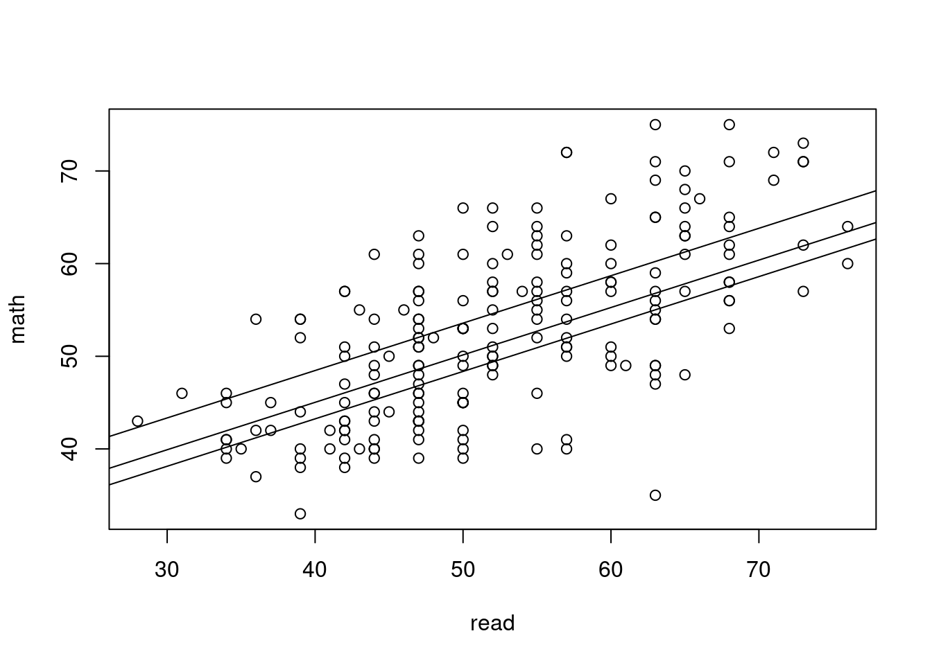
For example, a scatterplot can be specified as a formula with
the plot() function. Where we can specify a formula we can
almost always also specify a data= parameter to point to the
source of the variables.
First, load some example data and look at it.
library(faraway)
data(hsb)
head(hsb)
id gender race ses schtyp prog read write math science socst
1 70 male white low public general 57 52 41 47 57
2 121 female white middle public vocation 68 59 53 63 61
3 86 male white high public general 44 33 54 58 31
4 141 male white high public vocation 63 44 47 53 56
5 172 male white middle public academic 47 52 57 53 61
6 113 male white middle public academic 44 52 51 63 61plot(math ~ read, data=hsb)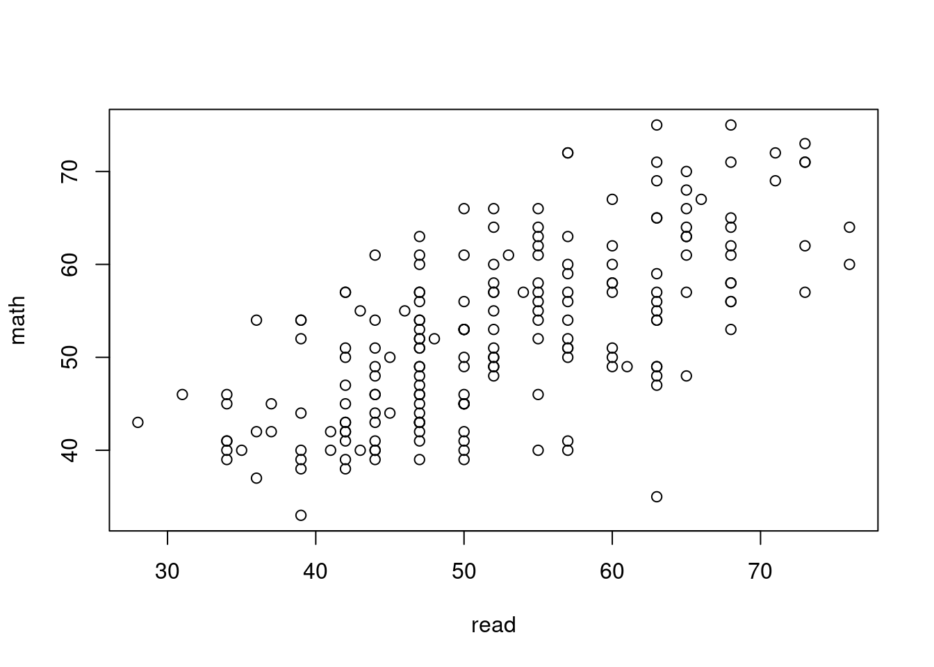
class(math ~ read)[1] "formula"20.2 T-test Formula
We have already seen formulas used in t-tests.
f <- formula(read ~ gender)
t.test(f, data=hsb)
    Welch Two Sample t-test

data:  read by gender
t = -0.74506, df = 188.46, p-value = 0.4572
alternative hypothesis: true difference in means between group female and group male is not equal to 0
95 percent confidence interval:
 -3.976725  1.796263
sample estimates:
mean in group female   mean in group male
            51.73394             52.82418
plot(f, data=hsb)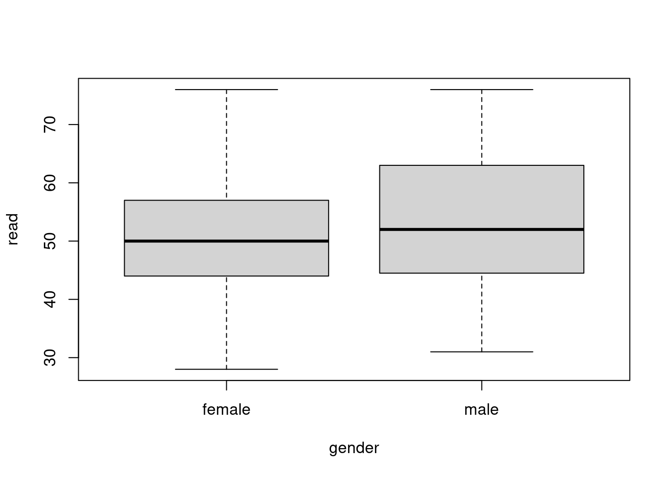
20.3 Linear Model Formula
Formulas are the central element in specifying regression models,
using lm() and a variety of other modeling functions.
20.3.1 Regression
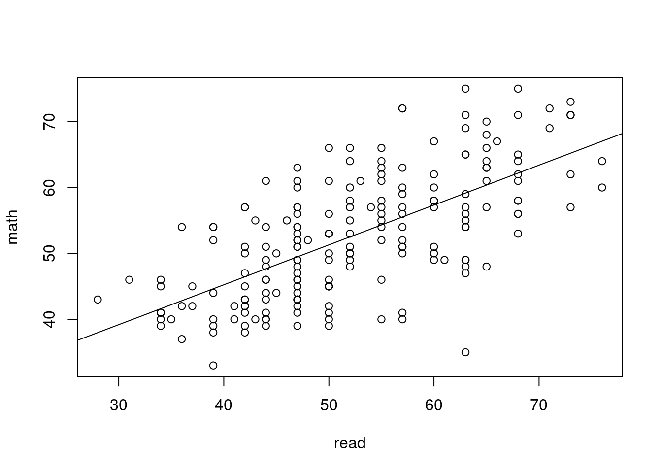
lm(math ~ read, data=hsb)
Call:
lm(formula = math ~ read, data = hsb)

Coefficients:
(Intercept)         read
    21.0382       0.6051
20.3.2 ANOVA
Anova models work in the same way.
plot(math ~ prog, data=hsb)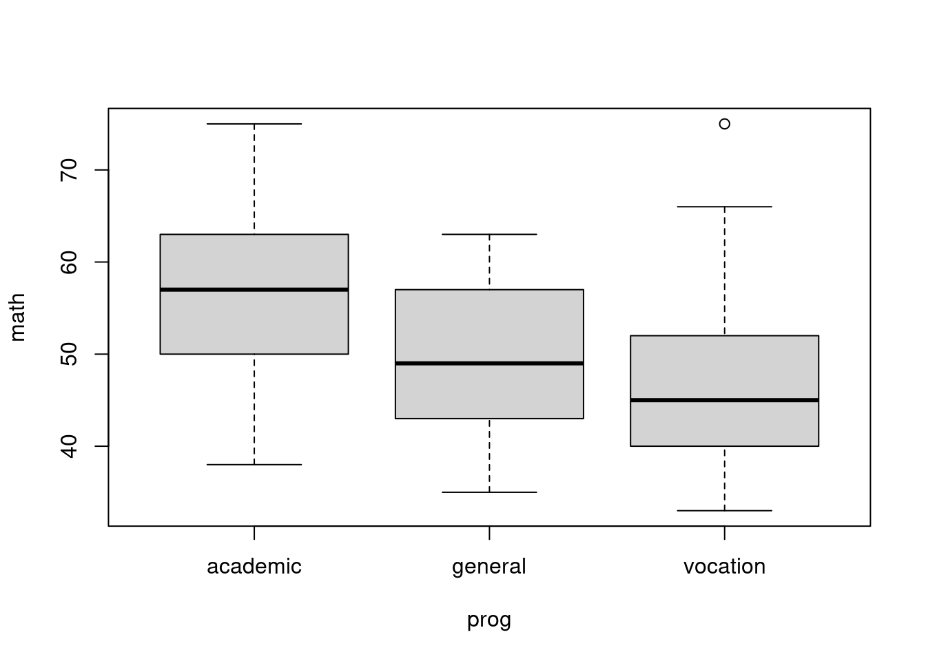
fit2 <- lm(math ~ prog, data=hsb)
summary(fit2)
Call:
lm(formula = math ~ prog, data = hsb)

Residuals:
     Min       1Q   Median       3Q      Max
-18.7333  -6.4200  -0.5767   6.2667  28.5800

Coefficients:
             Estimate Std. Error t value Pr(>|t|)
(Intercept)   56.7333     0.8068  70.321  < 2e-16 ***
proggeneral   -6.7111     1.4730  -4.556 9.12e-06 ***
progvocation -10.3133     1.4205  -7.260 8.73e-12 ***
---
Signif. codes:  0 '***' 0.001 '**' 0.01 '*' 0.05 '.' 0.1 ' ' 1

Residual standard error: 8.267 on 197 degrees of freedom
Multiple R-squared:  0.2291,    Adjusted R-squared:  0.2213
F-statistic: 29.28 on 2 and 197 DF,  p-value: 7.364e-12
Notice that the intercept is automatically included. While
prog is a single variable in our data it contributes two terms
to our model. R model formulae are similar to mathematical formulae,
but they are not the same thing.
20.3.3 Adding Variables Adds Terms
A model with more than one variable on the right-hand side:
library(magrittr)
lm(math ~ prog + read, data=hsb) %>%
  summary
Call:
lm(formula = math ~ prog + read, data = hsb)

Residuals:
     Min       1Q   Median       3Q      Max
-21.7994  -4.6484  -0.8686   4.8846  19.9834

Coefficients:
             Estimate Std. Error t value Pr(>|t|)
(Intercept)  27.99519    2.96929   9.428  < 2e-16 ***
proggeneral  -3.43297    1.24908  -2.748  0.00655 **
progvocation -5.21581    1.27015  -4.106  5.9e-05 ***
read          0.51170    0.05155   9.927  < 2e-16 ***
---
Signif. codes:  0 '***' 0.001 '**' 0.01 '*' 0.05 '.' 0.1 ' ' 1

Residual standard error: 6.761 on 196 degrees of freedom
Multiple R-squared:  0.487, Adjusted R-squared:  0.4792
F-statistic: 62.03 on 3 and 196 DF,  p-value: < 2.2e-16
20.3.4 Interaction Terms
Interactions may be specified a couple of different ways. An
asterisk, *, means to include the higher order term plus all
the related lower order terms. Alternatively, specific interaction
terms may be specified with the colon, :.
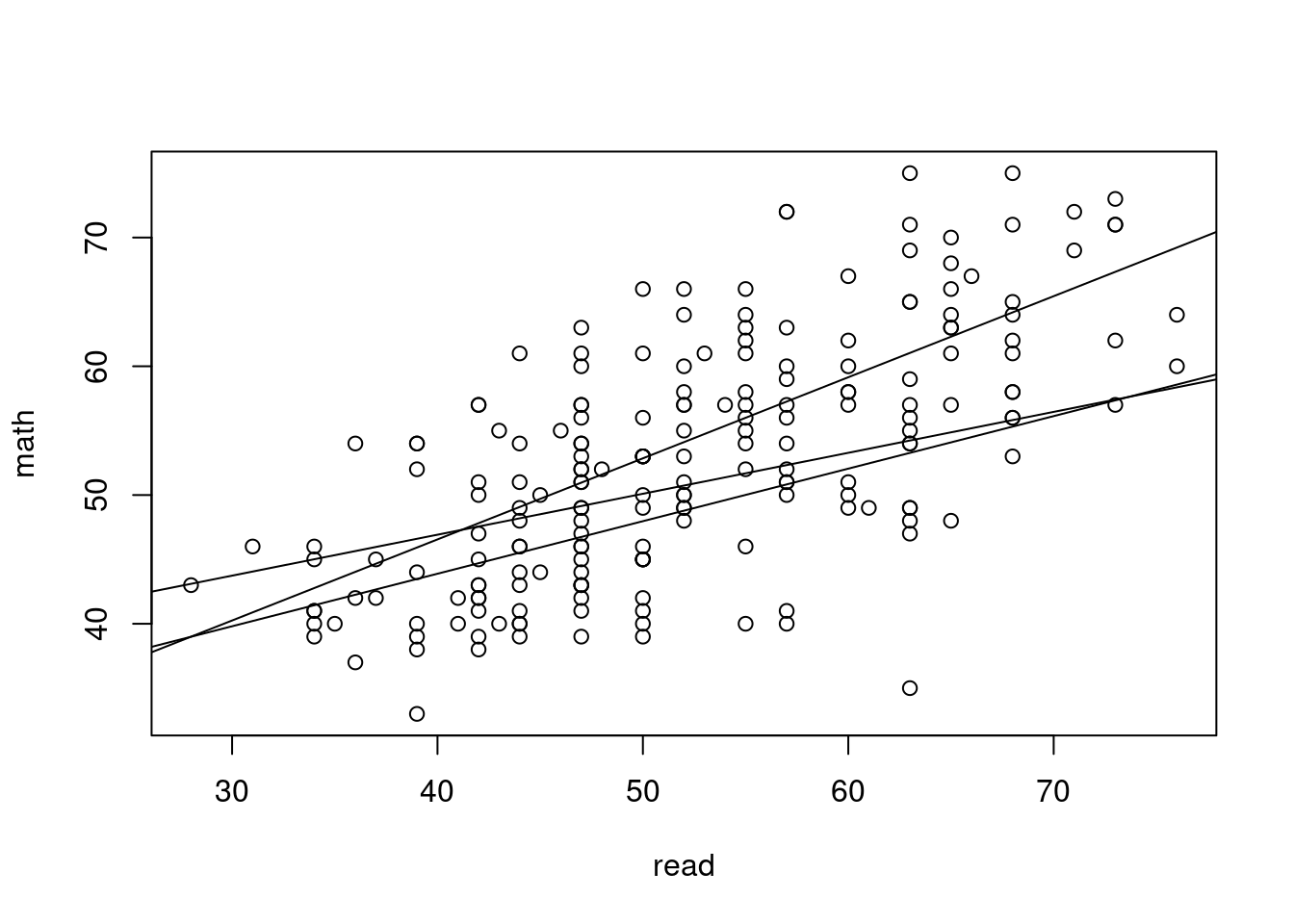
lm(math ~ prog * read, data=hsb)
Call:
lm(formula = math ~ prog * read, data = hsb)

Coefficients:
      (Intercept)        proggeneral       progvocation               read   proggeneral:read  progvocation:read
          21.3612            12.8386             6.2033             0.6298            -0.3118            -0.2217
# the same model, written out
lm(math ~ prog + read + prog:read, data=hsb)
Call:
lm(formula = math ~ prog + read + prog:read, data = hsb)

Coefficients:
      (Intercept)        proggeneral       progvocation               read   proggeneral:read  progvocation:read
          21.3612            12.8386             6.2033             0.6298            -0.3118            -0.2217
Here again, the variable prog contributes multiple terms,
and the interaction prog:read contributes multiple interaction
terms.
20.3.5 Updates for Formulas
Models may be modified - terms added or removed - through
the use of the update() function. In this context, a
period, ., represents all the terms included in the previous
model.
m1 <- lm(math ~ prog * read, data=hsb)
m1
Call:
lm(formula = math ~ prog * read, data = hsb)

Coefficients:
      (Intercept)        proggeneral       progvocation               read   proggeneral:read  progvocation:read
          21.3612            12.8386             6.2033             0.6298            -0.3118            -0.2217
update(m1, . ~ . -prog:read) # removes two model terms
Call:
lm(formula = math ~ prog + read, data = hsb)

Coefficients:
 (Intercept)   proggeneral  progvocation          read
     27.9952       -3.4330       -5.2158        0.5117
In a formula, a minus sign, -, is used to remove a term from
a model.
20.3.6 Inhibit Formula Interpretation
In formulas, the plus sign, +, means to add terms, but
we may also want to represent simple element-wise addition
of vectors in a formula.
For example, one way to constrain
the coefficients of several model terms to be equal is to
combine the variables into a single model term. To do this,
we use the inhibit function, I(). Expressions within the
I() function are interpreted as general R expressions, and
not as terms within the formula.
m3 <- lm(math ~ read+write+science+socst, hsb)
coefficients(m3) # to see why we might think some are equal
(Intercept) read write science socst
8.96274058 0.27068453 0.22616140 0.25389639 0.08480508 m4 <- lm(math ~ I(read+write+science)+socst, hsb)
anova(m4, m3) # An F test for difference between modelsAnalysis of Variance Table
Model 1: math ~ I(read + write + science) + socst
Model 2: math ~ read + write + science + socst
Res.Df RSS Df Sum of Sq F Pr(>F)
1 197 7699.2
2 195 7691.3 2 7.9174 0.1004 0.904620.3.7 Polynomials
R does not use the asterisk or colon to form tensor products like other software does. This limitation means we cannot create polynomial terms the same way we create interaction terms
lm(math ~ read + read:read, data=hsb) # no good
Call:
lm(formula = math ~ read + read:read, data = hsb)

Coefficients:
(Intercept)         read
    21.0382       0.6051
lm(math ~ read + I(read*read), data=hsb) # but this works
Call:
lm(formula = math ~ read + I(read * read), data = hsb)

Coefficients:
   (Intercept)            read  I(read * read)
     24.056044        0.487359        0.001106
lm(math ~ read + I(read^2), data=hsb) # and this works
Call:
lm(formula = math ~ read + I(read^2), data = hsb)

Coefficients:
(Intercept)         read    I(read^2)
  24.056044     0.487359     0.001106
(Orthogonal polynomials and centered data are often used when polynomial terms are of interest.)
20.3.8 Limiting higher order interactions
Often second-order interaction terms are of interest, while higher order terms are not.
lm(math ~ read*write*science, data=hsb) %>%
  summary
Call:
lm(formula = math ~ read * write * science, data = hsb)

Residuals:
     Min       1Q   Median       3Q      Max
-20.9229  -4.2197  -0.0111   4.3823  15.4383

Coefficients:
                     Estimate Std. Error t value Pr(>|t|)
(Intercept)         4.859e+01  6.982e+01   0.696    0.487
read               -2.603e-02  1.505e+00  -0.017    0.986
write              -7.682e-01  1.373e+00  -0.560    0.576
science             1.251e-02  1.382e+00   0.009    0.993
read:write          1.143e-02  2.851e-02   0.401    0.689
read:science       -4.338e-03  2.873e-02  -0.151    0.880
write:science       1.027e-02  2.632e-02   0.390    0.697
read:write:science -2.295e-05  5.301e-04  -0.043    0.966

Residual standard error: 6.237 on 192 degrees of freedom
Multiple R-squared:  0.5724,    Adjusted R-squared:  0.5568
F-statistic: 36.71 on 7 and 192 DF,  p-value: < 2.2e-16
lm(math ~ (read+write+science)^2, data=hsb) %>%
summary
Call:
lm(formula = math ~ (read + write + science)^2, data = hsb)

Residuals:
     Min       1Q   Median       3Q      Max
-20.8834  -4.2061  -0.0184   4.3747  15.4367

Coefficients:
               Estimate Std. Error t value Pr(>|t|)
(Intercept)   45.647268  15.589767   2.928  0.00382 **
read           0.036840   0.396119   0.093  0.92600
write         -0.711032   0.371207  -1.915  0.05691 .
science        0.070291   0.359881   0.195  0.84535
read:write     0.010230   0.006507   1.572  0.11755
read:science  -0.005555   0.005968  -0.931  0.35318
write:science  0.009163   0.006329   1.448  0.14931
---
Signif. codes:  0 '***' 0.001 '**' 0.01 '*' 0.05 '.' 0.1 ' ' 1

Residual standard error: 6.221 on 193 degrees of freedom
Multiple R-squared:  0.5724,    Adjusted R-squared:  0.5591
F-statistic: 43.05 on 6 and 193 DF,  p-value: < 2.2e-16
20.4 Table Formulas
The terms in a table formula serve to define the combinations of categories to be counted.
In individual level data, there is no left-hand side.
xtabs( ~ gender + schtyp, data=hsb) schtyp
gender private public
female 18 91
male 14 77In grouped data, the frequency counts are given on the left-hand side.
gender <- c("f","f","m","m")
schtyp <- c("pri","pub","pri","pub")
freq   <- c(18, 91, 14, 77)

df <- data.frame(gender, schtyp, freq)
df
gender schtyp freq
1 f pri 18
2 f pub 91
3 m pri 14
4 m pub 77xtabs(freq ~ gender + schtyp, data=df) schtyp
gender pri pub
f 18 91
m 14 77