 Supporting Statistical Analysis for Research
6.3 Aggregating data
6.3.1 Data concepts
Data aggregation is reducing a set of values to a smaller set of values (typically a single value) value through some function of the individual values. A common statistical data aggregation is reducing a distribution of values to a mean and standard deviation. Another example of data reduction is frequency tables.
Aggregating data is a useful tool for data exploration. A histogram is an example of aggregation for exploration. Histograms count (aggregate) the number of observations that fall into bins. While some data is lost in this aggregation, it also provides a very useful visualization of the distribution of a set of values.
Aggregation is sometimes done to allow for analysis to be completed at a higher level of the data. For example, if an analysis of the size of school districts in a region is to be done, the number of students from the schools with in the district are summed (aggregated.)
6.3.2 Examples - R
These examples use the Blackmore.csv data set.
We begin by loading the tidyverse and import the csv file.
library(tidyverse)blackmore_path <- file.path("..", "datasets", "Blackmore.csv") blackmore_in <- read_csv(blackmore_path, col_types = cols())Warning: Missing column names filled in: 'X1' [1]blackmore <- blackmore_in %>% select(-X1) glimpse(blackmore)Observations: 945 Variables: 4 $ subject <chr> "100", "100", "100", "100", "100", "101", "101", "101... $ age <dbl> 8.00, 10.00, 12.00, 14.00, 15.92, 8.00, 10.00, 12.00,... $ exercise <dbl> 2.71, 1.94, 2.36, 1.54, 8.63, 0.14, 0.14, 0.00, 0.00,... $ group <chr> "patient", "patient", "patient", "patient", "patient"...Some of the ages have fractional components. We will round down, the floor function, the
agevariable to find each subjects integer age.blackmore <- blackmore %>% mutate( age = floor(age) ) glimpse(blackmore)Observations: 945 Variables: 4 $ subject <chr> "100", "100", "100", "100", "100", "101", "101", "101... $ age <dbl> 8, 10, 12, 14, 15, 8, 10, 12, 14, 16, 8, 10, 12, 15, ... $ exercise <dbl> 2.71, 1.94, 2.36, 1.54, 8.63, 0.14, 0.14, 0.00, 0.00,... $ group <chr> "patient", "patient", "patient", "patient", "patient"...Find the mean
exercisebygroup, the treatment variable.mean_exercise <- blackmore %>% group_by( group ) %>% summarize(mean = mean(exercise)) mean_exercise %>% as.data.frame()group mean 1 control 1.640641 2 patient 3.075887The use of
as.data.frame()was used here to provide a more table like display.The mean within the treatment groups might vary over subject age. We will find the mean
exerciseby treatment and the last year a subject was in the program.last_age <- blackmore %>% group_by( subject ) %>% filter( age == max(age) ) %>% ungroup() mean_last_age_exercise <- last_age %>% group_by(group, age) %>% summarize(mean = mean(exercise)) mean_last_age_exercise %>% as.data.frame()group age mean 1 control 11 1.520000 2 control 12 1.730714 3 control 13 1.424545 4 control 14 2.381875 5 control 15 2.240588 6 control 16 2.505000 7 control 17 2.124444 8 patient 11 1.840000 9 patient 12 6.096000 10 patient 13 5.124211 11 patient 14 5.185667 12 patient 15 8.282857 13 patient 16 5.473488 14 patient 17 6.395000The way the data is displayed makes it difficult to compare the two groups. We will put the two groups into side by side columns in a table.
mean_last_age_exercise <-
  last_age %>%
  group_by(group, age) %>%
  summarize(mean = mean(exercise)) %>%
  spread(key = group, value = mean)

mean_last_age_exercise %>%
  as.data.frame()
age control patient 1 11 1.520000 1.840000 2 12 1.730714 6.096000 3 13 1.424545 5.124211 4 14 2.381875 5.185667 5 15 2.240588 8.282857 6 16 2.505000 5.473488 7 17 2.124444 6.395000We will repeat the prior problem and including the number of subjects in each group.
mean_last_age_exercise <-
  last_age %>%
  group_by(
    group,
    age
    ) %>%
  summarise(
    mean = mean(exercise),
    number = n()
    ) %>%
  gather(key = stat, value = value, mean, number) %>%
  unite(stat_name, sep = "-", group, stat) %>%
  spread(key = stat_name, value = value)

mean_last_age_exercise %>%
  as.data.frame()
age control-mean control-number patient-mean patient-number 1 11 1.520000 1 1.840000 1 2 12 1.730714 14 6.096000 5 3 13 1.424545 22 5.124211 19 4 14 2.381875 16 5.185667 30 5 15 2.240588 17 8.282857 28 6 16 2.505000 14 5.473488 43 7 17 2.124444 9 6.395000 12Make a histogram of the distribution of the size of the last age when grouped by age and treatment.
blackmore_group_size <-
  last_age %>%
  group_by(
    group,
    age
    ) %>%
  summarise(
    count = n()
    ) %>%
  ungroup()

ggplot(blackmore_group_size, aes(x = count)) +
  geom_histogram(binwidth = 1) +
  theme_bw()
6.3.3 Examples - Python
These examples use the Blackmore.csv data set.
We begin by loading the packages and importing the csv file.
import pandas as pd
import os
import numpy as np
blackmore_path = os.path.join('..', 'datasets', 'blackmore.csv') blackmore_in = pd.read_csv(blackmore_path) blackmore = ( blackmore_in .copy(deep=True) .drop(columns='Unnamed: 0')) (blackmore .head() .pipe(print))subject age exercise group 0 100 8.00 2.71 patient 1 100 10.00 1.94 patient 2 100 12.00 2.36 patient 3 100 14.00 1.54 patient 4 100 15.92 8.63 patientSome of the ages have fractional components. We will round down, the floor function, the
agevariable to find each subjects integer age.blackmore = ( blackmore .assign(age=lambda df: np.floor(df['age']).astype('int'))) (blackmore .head() .pipe(print))subject age exercise group 0 100 8 2.71 patient 1 100 10 1.94 patient 2 100 12 2.36 patient 3 100 14 1.54 patient 4 100 15 8.63 patientFind the mean
exercisebygroup, the treatment variable.The
mean()method for theGroupByobject will calculate the mean for each group. This is one of the aggregating methods forGroupBy.mean_exercise = ( blackmore .groupby('group') ['exercise'] .mean() .reset_index()) (mean_exercise .pipe(print))group exercise 0 control 1.640641 1 patient 3.075887The mean within the treatment groups might vary over subject age. We will find the mean
exerciseby treatment and the last year a subject was in the program.To find the last age for each participant, we sort by age and use the
tail()method to retain only the largest age.last_age = ( blackmore .sort_values(['subject', 'age']) .groupby('subject') .tail(1) .reset_index() ) mean_last_age_exercise = ( last_age .groupby(['group', 'age']) ['exercise'] .mean() .reset_index() ) (mean_last_age_exercise .pipe(print))group age exercise 0 control 11 1.520000 1 control 12 1.730714 2 control 13 1.424545 3 control 14 2.381875 4 control 15 2.240588 5 control 16 2.505000 6 control 17 2.124444 7 patient 11 1.840000 8 patient 12 6.096000 9 patient 13 5.124211 10 patient 14 5.185667 11 patient 15 8.282857 12 patient 16 5.473488 13 patient 17 6.395000The way the data is displayed makes it difficult to compare the two groups. We will put the two groups into side by side columns in a table.
mean_last_age_exercise = (
    last_age
        .groupby(['group', 'age'])
        ['exercise']
        .mean()
        .reset_index()
        .pivot(index='age', columns='group', values='exercise')
        )

(mean_last_age_exercise
   .pipe(print))
group control patient age 11 1.520000 1.840000 12 1.730714 6.096000 13 1.424545 5.124211 14 2.381875 5.185667 15 2.240588 8.282857 16 2.505000 5.473488 17 2.124444 6.395000We will repeat the prior problem and including the number of subjects in each group.
The built in aggregating functions for the
GroupByobject are useful if you need a single aggregating function for each group. Theaggregate()method is a more general purpose approach to aggregating data in groups. It is given a dictionary with an entry for each column that will have a aggregating function applied to it. A list of aggregating functions is given for each of the columns being aggregated.The
aggregate()method returns a column index in two rows (hierachtical index) when multiple functions are applied to a column.mean_last_age_exercise = ( last_age .groupby(['group', 'age']) .aggregate( {'exercise': ['mean', 'size']}) .reset_index() .rename_axis(None, axis='index') ) print(mean_last_age_exercise.head())group age exercise mean size 0 control 11 1.520000 1 1 control 12 1.730714 14 2 control 13 1.424545 22 3 control 14 2.381875 16 4 control 15 2.240588 17flat_col = [t[0] if t[1] == '' else t[1] for t in mean_last_age_exercise.columns] print(flat_col)['group', 'age', 'mean', 'size']mean_last_age_exercise.columns = flat_col mean_last_age_exercise = ( mean_last_age_exercise .pivot( index='age', columns='group', values=['mean', 'size']) .reset_index() .rename_axis(None, axis='index') ) print(mean_last_age_exercise.head())age mean size group control patient control patient 0 11 1.520000 1.840000 1.0 1.0 1 12 1.730714 6.096000 14.0 5.0 2 13 1.424545 5.124211 22.0 19.0 3 14 2.381875 5.185667 16.0 30.0 4 15 2.240588 8.282857 17.0 28.0flat_col = [ t[0] if t[1] == '' else t[1] + '-' + t[0] for t in mean_last_age_exercise.columns] print(flat_col)['age', 'control-mean', 'patient-mean', 'control-size', 'patient-size']mean_last_age_exercise.columns = flat_col (mean_last_age_exercise .pipe(print))age control-mean patient-mean control-size patient-size 0 11 1.520000 1.840000 1.0 1.0 1 12 1.730714 6.096000 14.0 5.0 2 13 1.424545 5.124211 22.0 19.0 3 14 2.381875 5.185667 16.0 30.0 4 15 2.240588 8.282857 17.0 28.0 5 16 2.505000 5.473488 14.0 43.0 6 17 2.124444 6.395000 9.0 12.0Make a histogram of the distribution of the size of the last age when grouped by age and treatment.
last_age_group_size = (
    last_age
        .groupby(['group', 'age'])
        ['exercise']
        .size()
        .reset_index()
        .rename(columns={'exercise': 'size'})
        )
print(last_age_group_size.head())
group age size 0 control 11 1 1 control 12 14 2 control 13 22 3 control 14 16 4 control 15 17(p9.ggplot(last_age_group_size, p9.aes(x='size')) + p9.geom_histogram(binwidth=1) + p9.theme_bw())<ggplot: (-9223371893255862198)>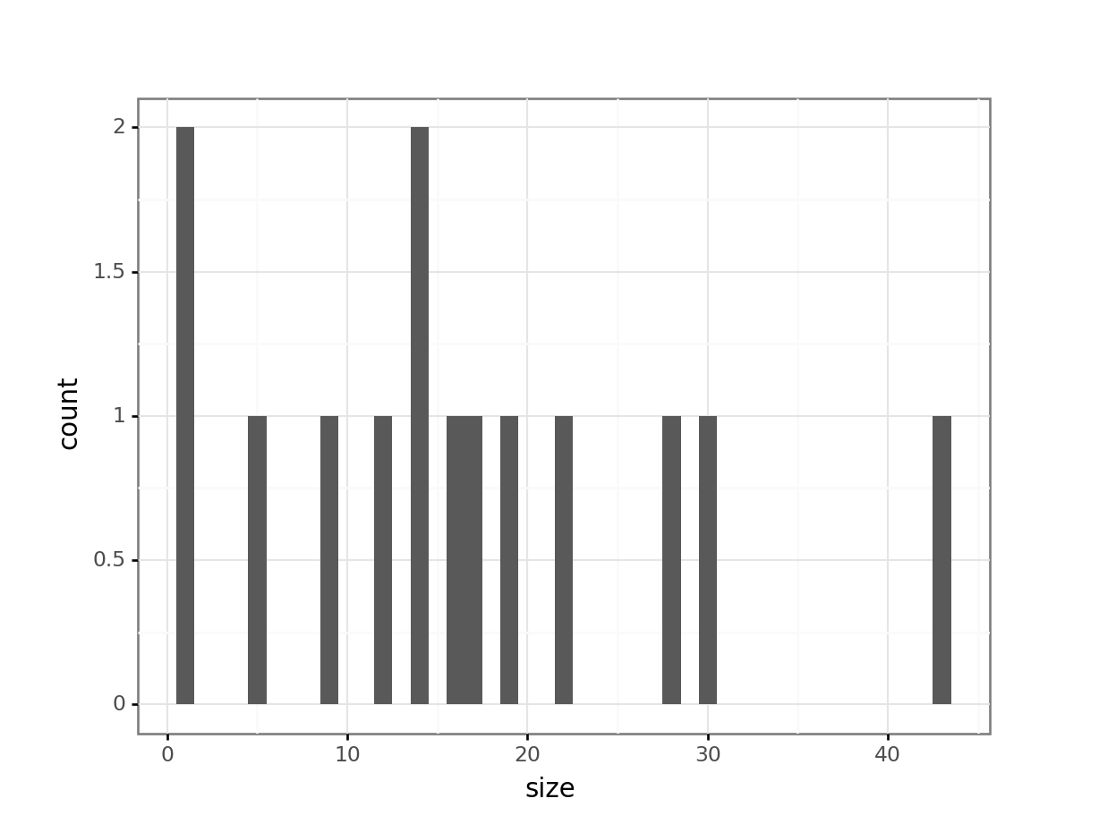
6.3.4 Exercises
These examples use the Car.csv data set.
Load the
Car.csvdata set.Create a categorical variable that identifies the body type that was selected first.
Create a table of the number of count of the selected types.
Create a table of the number of trucks selected by college degree or not and greater than 2 in the family.
Which of these subgroups selected
truckas their first choice in greatest numbers.Create the same table with the cells reporting the proportion of these groups that select trucks.
Which of these subgroups was most likely to selected
truckas their first choice.Create a variable that identifies the price of the first selected vehicle.
Create a table that provides the mean and standard deviation of price by college attendance or not groups.