4 Data Structure and Class

4.1 Warm-Up

The code below creates four objects, w, x, y, and z.

w <- 1:16
x <- w
dim(x) <- c(4, 4)
y <- as.data.frame(x)
z <- list(w, x, y)

All four objects contain the numbers 1-16, but they vary in their structure.

Print each one to the console.

Which objects are most similar to each other?
What is unique about each object?

Plot each one.

What is shown in each plot?

4.2 Outcomes

Objective: To explain the difference between the four basic data structures and the data types they can contain, and to check the class of an object.

Why it matters: Data wrangling, modeling, plotting, and programming all require you to construct, manipulate, and use different data structures, and an object’s structure and class determine how some functions behave.

Learning outcomes:

Fundamental Skills

Name how many data types different structures can contain.
View the structure of a data object.
Find the class(es) of an object.

Key functions and operators:

:
as.data.frame()
str()
class()

4.3 Four Structures

A data object’s structure refers to how it is organized (its “shape”). Different structures allow for varying diversity of data types. As we saw in the previous chapter, a vector can only contain a single type. Attempting to combine multiple types in a single vector results in implicit coercion.

The four basic structures in R are vectors, lists, matrices (and arrays), and dataframes. We can distinguish them by their number of dimensions the number of types they can contain:

Structure	Dimensions	Types
vector	1	1
list	1	1+
matrix	2	1
dataframe	2	1+

Vectors are composed of one or more elements (values), all of the same type.

Lists are complex objects since they can contain other structures. In the warm-up, z (a list) contained w (a vector), x (a matrix), and y (a dataframe). Lists can also contain other lists and thus be nested. Lists are very flexible and convenient ways to store arbitrary sets of objects. When you fit a statistical model in R, it will return a list that contains a vector of residuals, a copy of the dataframe you used to fit the model, a nested list with the formula, and much more.

Matrices are two-dimensional and have only a single type. You will rarely encounter matrices in applied research and data wrangling, other than of correlation matrices in models and distance matrices in spatial data. Arrays are even less common; they can have three or more dimensions.

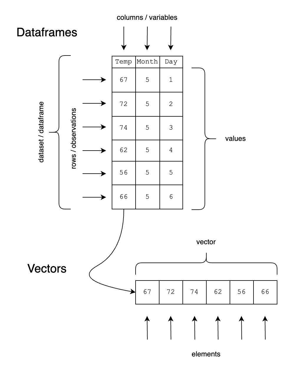
Dataframes are two-dimensional. They have rows (observations) and columns (variables). Each column in a dataframe is actually a vector. That means a dataframe is a collection of one or more same-length vectors. Each column/variable/vector can only contain a single type, but each column can be of a different type.

Most of our work in data wrangling will be with dataframes and vectors. We have various names for their parts, which you can find in the diagram below:

Tip

You may be anxious to start working with “real” data in the form of dataframes. If you look at the chapter navigation on the left, you will see that we have several chapters about vectors before we begin work with dataframes.

This is intentional. We will first learn skills to work with vectors of various kinds. These vectors will generally be short so that we can immediately see the effects of our code.

All the skills we learn with vectors will become relevant when working with dataframes, because dataframes are just lists of vectors. Anything we can do with a vector, we can do with a column in a dataframe.

Hang in there. We will work with dataframes soon!

4.4 Exploring Structures

We have many tools to explore our data objects:

Printing. Enter the name of an object in the console to see its contents:

 [1]  1  2  3  4  5  6  7  8  9 10 11 12 13 14 15 16

     [,1] [,2] [,3] [,4]
[1,]    1    5    9   13
[2,]    2    6   10   14
[3,]    3    7   11   15
[4,]    4    8   12   16

  V1 V2 V3 V4
1  1  5  9 13
2  2  6 10 14
3  3  7 11 15
4  4  8 12 16

[[1]]
 [1]  1  2  3  4  5  6  7  8  9 10 11 12 13 14 15 16

[[2]]
     [,1] [,2] [,3] [,4]
[1,]    1    5    9   13
[2,]    2    6   10   14
[3,]    3    7   11   15
[4,]    4    8   12   16

[[3]]
  V1 V2 V3 V4
1  1  5  9 13
2  2  6 10 14
3  3  7 11 15
4  4  8 12 16

str(). Use the str() function to see an object’s type(s), dimension sizes, and some of its values:

str(w)

 int [1:16] 1 2 3 4 5 6 7 8 9 10 ...

str(x)

 int [1:4, 1:4] 1 2 3 4 5 6 7 8 9 10 ...

str(y)

'data.frame':    4 obs. of  4 variables:
 $ V1: int  1 2 3 4
 $ V2: int  5 6 7 8
 $ V3: int  9 10 11 12
 $ V4: int  13 14 15 16

str(z)

List of 3
 $ : int [1:16] 1 2 3 4 5 6 7 8 9 10 ...
 $ : int [1:4, 1:4] 1 2 3 4 5 6 7 8 9 10 ...
 $ :'data.frame':    4 obs. of  4 variables:
  ..$ V1: int [1:4] 1 2 3 4
  ..$ V2: int [1:4] 5 6 7 8
  ..$ V3: int [1:4] 9 10 11 12
  ..$ V4: int [1:4] 13 14 15 16

For dataframes, we get the name and type of each column.

View(). For matrices, dataframes, and lists, run View(object_name). For matrices and dataframes, we can click on column names to sort the data. Note this does not actually change the order of the rows in the object itself. For smaller datasets, this can be a nice way to quickly browse the data. For lists, we get nested output where we can click on the blue triangles to iteratively explore the data.

Indexing. Use square brackets or dollar signs with position numbers or names.

Vectors: Use a vector (one or more numbers) to index a vector:

w[1] # first element

[1] 1

w[2:3] # second through third element

[1] 2 3

Matrices: Use one or two vectors to get rows, columns, or specific values:

x[1, ] # row 1, all columns

[1]  1  5  9 13

x[, 1] # all rows, column 1

[1] 1 2 3 4

x[2, 2] # row 2, column 2

[1] 6

x[2, 2:4] # row 2, columns 2-4

[1]  6 10 14

Dataframes: Use the same strategy as matrices, or use dataframe$column:
```
y$V2 # column V2
```
```
[1] 5 6 7 8
```

Lists: Use double square brackets in addition to the above strategies:

z[[1]] # first element, the vector

 [1]  1  2  3  4  5  6  7  8  9 10 11 12 13 14 15 16

z[[2]] # second element, the matrix

     [,1] [,2] [,3] [,4]
[1,]    1    5    9   13
[2,]    2    6   10   14
[3,]    3    7   11   15
[4,]    4    8   12   16

z[[2]][2,2] # row 2, column 2 of the second element

[1] 6

z[[3]] # third element, the dataframe

  V1 V2 V3 V4
1  1  5  9 13
2  2  6 10 14
3  3  7 11 15
4  4  8 12 16

z[[3]]$V2 # column V2 of the third element

[1] 5 6 7 8

4.5 Class

In R, data objects have one or more classes. Get an object’s class(es) with the class() function:

class(w)

[1] "integer"

class(x)

[1] "matrix" "array"

class(y)

[1] "data.frame"

class(z)

[1] "list"

Type, structure, and class are overlapping ways of describing our objects. The type and class of w are both integer. The structure and class of y are both dataframe. x has two classes, matrix and array.

What does class do? When we give an object to a function, the function will look at the object’s class. The function may do different things for objects of different classes, or it may return an error if an object does not have a certain class.

We saw that in the warm-up where plotting either two-dimensional arrangement of the data (the matrix x and the dataframe y) produced different plots, while trying to plot the list z resulted in an error.

You will usually encounter the issue of class when a function returns an error. In that case, check the documentation for the function you are using to see the object classes it supports.

4.6 Exercises

4.6.1 Fundamental

Use str() to explore these objects. What is each one’s structure? What type(s) do they contain?

Note: these objects are built in to R. They are available to your current session even though you do not see them in your environment. See ?Constants and help(package=datasets)
```
letters
month.name
pi
mtcars
penguins_raw
```
What are the structure and class(es) of the built-in state.x77 dataset? Plot it.

Change it into a dataframe with dat <- as.data.frame(state.x77). What are the structure and class(es) of dat? Plot it.