9 Categorical Vectors

9.1 Warm-Up

Use this line of code to create a categorical variable object, y.

y <- factor(c("a", "b", "c", "b", "d", "a", "a"))

Use the functions str() and plot() to explore the object.

What do you notice about the order of the letters we gave to factor() and the order returned by str() and plot()?
Change the order of the letters in the code. Then use str() and plot() again. What do you notice now?

9.2 Outcomes

Objective: To create factor vectors from other vectors and manipulate factors by changing their orders, labels, and levels.

Why it matters: Factors provide a way to include character data in modeling and plotting, and manipulating factors can change things like intercept and interaction terms in models, and axis orders in plots.

Learning outcomes:

Fundamental Skills	Extended Skills
Create a factor vector from another vector. Change the order of a factor’s levels. Change the labels of a factor’s levels. Reduce the number of levels in a factor by combining them.	Apply a function to change the labels of a factor’s levels. Recode a numeric vector into a factor.

Key functions:

factor()
levels()
fct_relevel()
fct_recode()
fct_relabel()
fct_collapse()

9.3 Factors

We can divide data into two general categories: continuous and categorical. Continuous data is numeric, has a natural order, and can potentially take on an infinite number of values. Examples include age, income, and health care expenditures. In contrast, categorical data takes on a limited number of values and may or may not have a natural order. Examples without a natural order include race, state of residence, and political affiliation. Examples with a natural order include Likert scale items (e.g., disagree, neutral, agree), socioeconomic status, and educational attainment.

The distinction between continuous and categorical variables is fundamental to how we use them in an analysis. For example, in a regression model, continuous variables give us slopes while categorical variables give us intercepts. If we want to use a variable as an outcome, we will have to decide whether to treat it as continuous or categorical (based on its distribution and number of observed values). If it is categorical, we need to decide whether it is ordered (for an ordinal logistic regression) or unordered (for a multinomial logistic regression).

In R, categorical data is managed as factors. We specify which variables are factors when we create and store them, and then they are treated as categorical variables in a model without any additional specification. This contrasts with other software like Stata, SAS, and SPSS, where we specify which variables are categorical in our model syntax.

9.3.1 Structure

Understanding how R represents factors will help us understand how to manipulate them.

Begin with a simple character vector, x, that contains the letters a, b, c, and d.

x <- c("a", "b", "c", "b", "d", "a", "a")

When we print x, R quotes the values:

[1] "a" "b" "c" "b" "d" "a" "a"

Now, make a factor called y from x with the factor() function:

y <- factor(x)
y

[1] a b c b d a a
Levels: a b c d

y prints differently than x. It does not have quotes around its values, and it contains a line about something called “levels,” which contains the unique values of y.

A factor is composed of two parts: an integer vector and an ordered label vector. To see the underlying integer vector of y, we can coerce it to numeric with as.numeric():

as.numeric(y)

[1] 1 2 3 2 4 1 1

And we can see the ordered labels with the levels() function:

levels(y)

[1] "a" "b" "c" "d"

The label “a” is the first level, “b” the second, “c” the third, and “d” the fourth. Factor levels are ordered alphabetically by default. We could make a key as follows:

Integer	Label
1	a
2	b
3	c
4	d

Now, our y factor is actually an integer vector, but when we print it, R shows the corresponding labels.

Compare the output from y and as.numeric(y) once again, and refer to the table above.

[1] a b c b d a a
Levels: a b c d

as.numeric(y)

[1] 1 2 3 2 4 1 1

9.3.2 Defaults

When we include a character variable when plotting or modeling in R, R treats it as a factor, and its defaults are to

sort levels alphabetically by their label
leave the existing labels as-is
include all unique values

Why are these problems?

To see why this is not ideal, simulate some survey response data, where individuals could indicate whether they agreed, neither agreed nor disagreed, or disagreed with a statement, or if the statement did not apply to them (“not applicable”). Individuals could also choose to not answer the question (“no answer”).

answers <- c("AGREE", 
             "NEITHER",
             "DISAGREE",
             "NOT APPLICABLE",
             "NO ANSWER")
responses <- factor(sample(answers, 100, replace = T))

Now, make a plot of counts by response.

ggplot() +
  geom_bar(aes(x = responses))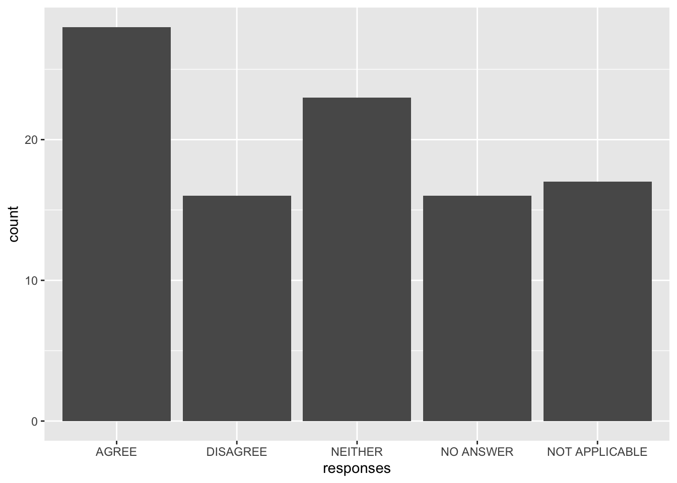

(To learn more about how to use ggplot, see Data Visualization in R.)

We can see R’s defaults in action:

The levels were ordered alphabetically, but it would make more sense to have “neither” between “agree” and “disagree.”
The labels were used as-is, but we might choose to not use all-uppercase labels to improve the appearance of the plot (e.g., “Agree” rather than “AGREE”).
All values in our data were included, but we might consider combining the two categories of “no answer” and “not applicable” to a single “missing.”

We will learn how to manipulate these three aspects of factors in R: order (releveling), labels (recoding), and number of categories (collapsing). For all of these operations, we will be making use of the forcats library from the tidyverse, which makes it easy to manipulate factors.

9.4 Releveling

When we relevel a factor, we change the order of its levels. If we give fct_relevel() the name of a factor and the name of a level, it moves that level to the first position and leaves the others in their current order.

First, load the tidyverse.

library(tidyverse)

Using y from earlier, create y_relevel, which has “b” instead of “a” as its first level.

y_relevel <- fct_relevel(y, "b")

The levels of y_relevel are as follows:

Integer	Label
1	b
2	a
3	c
4	d

Compare the output from y and y_relevel when printing them as is, printing their underlying integers, and printing their levels.

[1] a b c b d a a
Levels: a b c d

y_relevel

[1] a b c b d a a
Levels: b a c d

as.numeric(y)

[1] 1 2 3 2 4 1 1

as.numeric(y_relevel)

[1] 2 1 3 1 4 2 2

levels(y)

[1] "a" "b" "c" "d"

levels(y_relevel)

[1] "b" "a" "c" "d"

The data still prints the same, but the order of the levels has changed, and this is reflected in the integer output. In y_relevel, “b” is 1 and “a” is 2.

9.4.1 Changing the Reference Level

We can use R’s built-in penguins dataset, which has data on penguins from Antarctica. It has 3 factor variables and 5 numeric variables.

str(penguins)

'data.frame':   344 obs. of  8 variables:
 $ species    : Factor w/ 3 levels "Adelie","Chinstrap",..: 1 1 1 1 1 1 1 1 1 1 ...
 $ island     : Factor w/ 3 levels "Biscoe","Dream",..: 3 3 3 3 3 3 3 3 3 3 ...
 $ bill_len   : num  39.1 39.5 40.3 NA 36.7 39.3 38.9 39.2 34.1 42 ...
 $ bill_dep   : num  18.7 17.4 18 NA 19.3 20.6 17.8 19.6 18.1 20.2 ...
 $ flipper_len: int  181 186 195 NA 193 190 181 195 193 190 ...
 $ body_mass  : int  3750 3800 3250 NA 3450 3650 3625 4675 3475 4250 ...
 $ sex        : Factor w/ 2 levels "female","male": 2 1 1 NA 1 2 1 2 NA NA ...
 $ year       : int  2007 2007 2007 2007 2007 2007 2007 2007 2007 2007 ...

The first, or reference, level of island is “Biscoe”:

levels(penguins$island)

[1] "Biscoe"    "Dream"     "Torgersen"

If we make box plots of flipper length (flipper_len) by island, we see that “Biscoe” is the first value on the x-axis:

plot(flipper_len ~ island, penguins)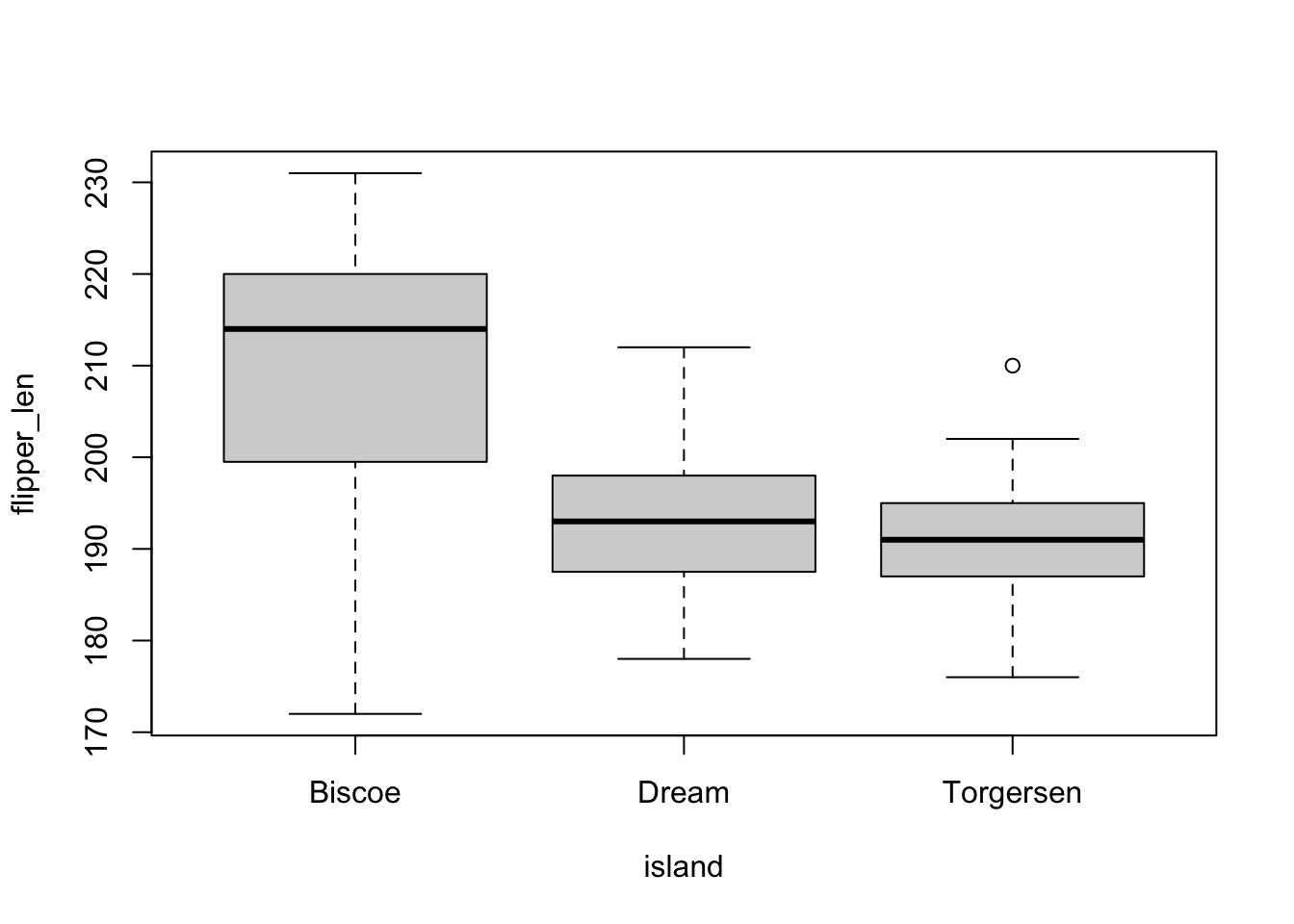

And if we predict flipper_len by island in a linear model, we will get this output:

summary(lm(flipper_len ~ island, penguins))


Call:
lm(formula = flipper_len ~ island, data = penguins)

Residuals:
    Min      1Q  Median      3Q     Max 
-37.707  -5.196   1.804   6.927  21.293 

Coefficients:
                Estimate Std. Error t value Pr(>|t|)    
(Intercept)     209.7066     0.8621  243.25   <2e-16 ***
islandDream     -16.6340     1.3207  -12.60   <2e-16 ***
islandTorgersen -18.5105     1.7824  -10.38   <2e-16 ***
---
Signif. codes:  0 '***' 0.001 '**' 0.01 '*' 0.05 '.' 0.1 ' ' 1

Residual standard error: 11.14 on 339 degrees of freedom
  (2 observations deleted due to missingness)
Multiple R-squared:  0.376, Adjusted R-squared:  0.3723 
F-statistic: 102.1 on 2 and 339 DF,  p-value: < 2.2e-16

Our reference level, Biscoe, is omitted since it is represented by the intercept. The other islands’ coefficients are comparisons to the reference category, or adjustments to the intercept. In R model output, the coefficients for the levels of a factor variable are labeled with the variable name followed by the level label, so the coefficient for the Dream level of the island variable is called islandDream.

If we want to change the ordering of a categorical variable in a plot or change the reference level in a statistical model, we need to relevel our factor. We can make another variable in penguins called island_relevel where “Dream” is the reference level:

penguins$island_relevel <- fct_relevel(penguins$island, "Dream")

Now, if we plot flipper_len by island with island_relevel, “Dream” is the first value on the x-axis, followed by “Biscoe” and “Torgersen.”

plot(flipper_len ~ island_relevel, penguins)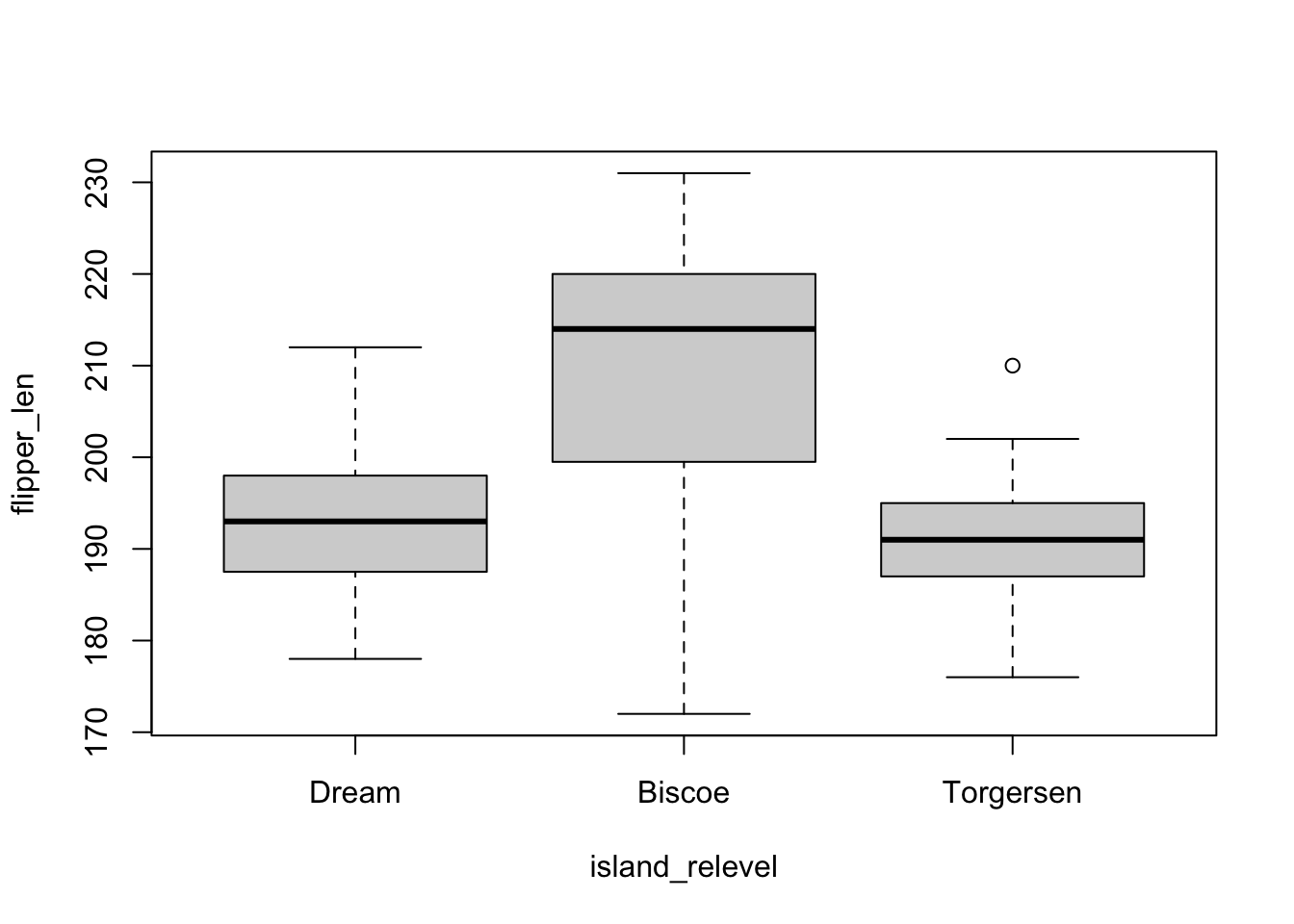

And if we fit our model again with island_relevel, we see that the intercept has changed since it now represents the expected value of flipper_len when the island is set to Dream.

summary(lm(flipper_len ~ island_relevel, penguins))


Call:
lm(formula = flipper_len ~ island_relevel, data = penguins)

Residuals:
    Min      1Q  Median      3Q     Max 
-37.707  -5.196   1.804   6.927  21.293 

Coefficients:
                        Estimate Std. Error t value Pr(>|t|)    
(Intercept)              193.073      1.000 192.983   <2e-16 ***
island_relevelBiscoe      16.634      1.321  12.595   <2e-16 ***
island_relevelTorgersen   -1.877      1.853  -1.013    0.312    
---
Signif. codes:  0 '***' 0.001 '**' 0.01 '*' 0.05 '.' 0.1 ' ' 1

Residual standard error: 11.14 on 339 degrees of freedom
  (2 observations deleted due to missingness)
Multiple R-squared:  0.376, Adjusted R-squared:  0.3723 
F-statistic: 102.1 on 2 and 339 DF,  p-value: < 2.2e-16

If we want to calculate the expected value for Biscoe, we would add its coefficient to the intercept, and the result would match the intercept in our previous model.

For more on interpreting and visualizing regression models, see Visualizing Regression Results in R.

9.4.2 Changing All the Levels

So far we have only specified one level with fct_relevel(), but we can specify as many levels as we want. Anything we do not name will follow those we do name.

This is useful when our factor levels have a natural order, like responses on a Likert scale:

survey <- 
  factor(c("Strongly agree", 
           "Agree", 
           "Neither agree nor disagree",
           "Disagree",
           "Strongly disagree"))
levels(survey)

[1] "Agree"                      "Disagree"                  
[3] "Neither agree nor disagree" "Strongly agree"            
[5] "Strongly disagree"

survey <- 
  fct_relevel(survey,
              "Strongly disagree", 
              "Disagree", 
              "Neither agree nor disagree",
              "Agree",
              "Strongly agree")
levels(survey)

[1] "Strongly disagree"          "Disagree"                  
[3] "Neither agree nor disagree" "Agree"                     
[5] "Strongly agree"

9.5 Recoding

Recoding is changing the labels on our factors. To do this, we can supply fct_recode() with our factor and a series of "new_label" = "current_label" pairs. Anything we do not name will be left in its existing state.

Using y again, create y_recode, which has full fruit names instead of just their first letters:

y_recode <- 
  fct_recode(y,
             "apple" = "a",
             "banana" = "b",
             "cantaloupe" = "c",
             "durian" = "d")

The levels of y_recode are as follows:

Integer	Label
1	apple
2	banana
3	cantaloupe
4	durian

Only the labels of the data are changed when recoding. The order and the underlying numeric values remain the same.

[1] a b c b d a a
Levels: a b c d

y_recode

[1] apple      banana     cantaloupe banana     durian     apple      apple     
Levels: apple banana cantaloupe durian

as.numeric(y)

[1] 1 2 3 2 4 1 1

as.numeric(y_recode)

[1] 1 2 3 2 4 1 1

levels(y)

[1] "a" "b" "c" "d"

levels(y_recode)

[1] "apple"      "banana"     "cantaloupe" "durian"

With penguins, we can change how one or more levels are labeled. Abbreviate Torgersen to “Torg”:

penguins$island_recode <- 
  fct_recode(penguins$island, 
             "Torg" = "Torgersen")
levels(penguins$island)

[1] "Biscoe"    "Dream"     "Torgersen"

levels(penguins$island_recode)

[1] "Biscoe" "Dream"  "Torg"

Use the table() function after recoding to verify that the recoding worked as intended:

table(penguins$island, penguins$island_recode)

           
            Biscoe Dream Torg
  Biscoe       168     0    0
  Dream          0   124    0
  Torgersen      0     0   52

The first argument of table() (island) is the rows, and the second (island_recode) is the columns. To verify recoding, we only need to care whether the cells are zero or nonzero. We can see that wherever we had “Torgersen” in island, we have “Torg” in island_recode.

9.5.1 Make Levels Missing

Missing values can be coded with a variety of labels. To turn a level of a factor into missing, recode it as NULL.

All the corresponding values are converted to NA, and the level we made missing is removed from the levels() output.

Remove the level “b” from y:

y_miss <- fct_recode(y, NULL = "b")
y_miss

[1] a    <NA> c    <NA> d    a    a   
Levels: a c d

as.numeric(y_miss)

[1]  1 NA  2 NA  3  1  1

levels(y_miss)

[1] "a" "c" "d"

The levels of y_miss are as follows:

Integer	Label
1	a
2	c
3	d

9.5.2 Numeric Categorical Variables

Sometimes, variables appear to be continuous, numeric variables, but they are actually categorical variables.

An example of this is if we have Likert scale data. Responses may range 1-5 and represent level of agreement. Some may argue that we can treat such a variable as continuous, but for now we will force it to be categorical.

survey <- sample(1:5, 100, replace = T)

If we were to pass survey to fct_recode(), we will get an error:

survey <- 
  fct_recode(survey,
             "Strongly agree" = 1, 
             "Agree" = 2, 
             "Neither agree nor disagree" = 3,
             "Disagree" = 4,
             "Strongly disagree" = 5)

Error in `fct_recode()`:
! `.f` must be a factor or character vector, not an integer vector.

This is because fct_recode() (as well as all the other fct_*() functions) require a character or factor vector as the first argument (called .f). If we want to manipulate a numeric vector, we need to first coerce it to a character or factor before recoding it. Because its values/labels will then be characters, we need to quote the names of the existing levels (e.g., "1" rather than 1).

survey <- 
  fct_recode(as.character(survey),
             "Strongly agree" = "1", 
             "Agree" = "2", 
             "Neither agree nor disagree" = "3",
             "Disagree" = "4",
             "Strongly disagree" = "5")

9.6 Collapsing

Another factor manipulation is reducing the number of levels, called collapsing. Sometimes we have a factor with many levels, but very few observations exist at some levels. This can cause problems in estimation, especially in logistic regression models. We can combine levels with few observations together.

We can do this with fct_collapse(), and our arguments follow the pattern "new_level" = c("current_level_1", "current_level_2", ...).

We can combine levels from y so that “a” is in a new level called “vowel”, and the other three letters (“b”, “c”, and “d”) are combined into a group called “consonant.”

y_collapse <- 
  fct_collapse(y,
               "vowel" = "a",
               "consonant" = c("b", "c", "d"))

Our levels for y_collapse are now as follows:

Integer	Label
1	vowel
2	consonant

This process is irreversible since we have lost data granularity. We could change “vowel” back into “a” with fct_recode() since this level of y_collapse is only composed of one level from y. However, because “consonant” is a composite of multiple levels, it is impossible to separate this level back into “b”, “c”, and “d”. Therefore, it is a good idea to create a new object or variable when collapsing a factor.

Compare the output and structure of y and y_collapse to see how the data has changed:

[1] a b c b d a a
Levels: a b c d

y_collapse

[1] vowel     consonant consonant consonant consonant vowel     vowel    
Levels: vowel consonant

as.numeric(y)

[1] 1 2 3 2 4 1 1

as.numeric(y_collapse)

[1] 1 2 2 2 2 1 1

levels(y)

[1] "a" "b" "c" "d"

levels(y_collapse)

[1] "vowel"     "consonant"

After collapsing, we should compare the original and new factors to verify the coding worked as intended:

table(y, y_collapse)

   y_collapse
y   vowel consonant
  a     3         0
  b     0         2
  c     0         1
  d     0         1

Again, we only need to check whether the cells are zero or nonzero. The exact count does not matter. Here, all the values of “a” in y correspond to “vowel” in y_collapse, while all the values of “b”, “c”, and “d” correspond to “consonant.”

9.6.1 Empty Levels

If we take a subset of our data, the levels data for factor variables remains unchanged, even if we have excluded all observations at a certain level.

Take a subset of the first six rows (with head()) of penguins and store them as penguins_subset.

penguins_subset <- head(penguins)

The levels data for penguins_subset still includes all three islands, even though we only have “Torgersen” in our subset.

penguins_subset$island

[1] Torgersen Torgersen Torgersen Torgersen Torgersen Torgersen
Levels: Biscoe Dream Torgersen

as.numeric(penguins_subset$island)

[1] 3 3 3 3 3 3

levels(penguins_subset$island)

[1] "Biscoe"    "Dream"     "Torgersen"

This can have some annoying consequences for some plots, where levels with no observations are still included:

plot(flipper_len ~ island, penguins_subset)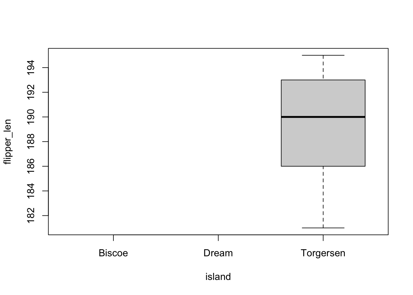

To remove these extra levels, simply use factor() to “reset” the factor and drop unused levels:

penguins_subset$island <- factor(penguins_subset$island)

Now verify that these levels were removed:

penguins_subset$island

[1] Torgersen Torgersen Torgersen Torgersen Torgersen Torgersen
Levels: Torgersen

as.numeric(penguins_subset$island)

[1] 1 1 1 1 1 1

levels(penguins_subset$island)

[1] "Torgersen"

plot(flipper_len ~ island, penguins_subset)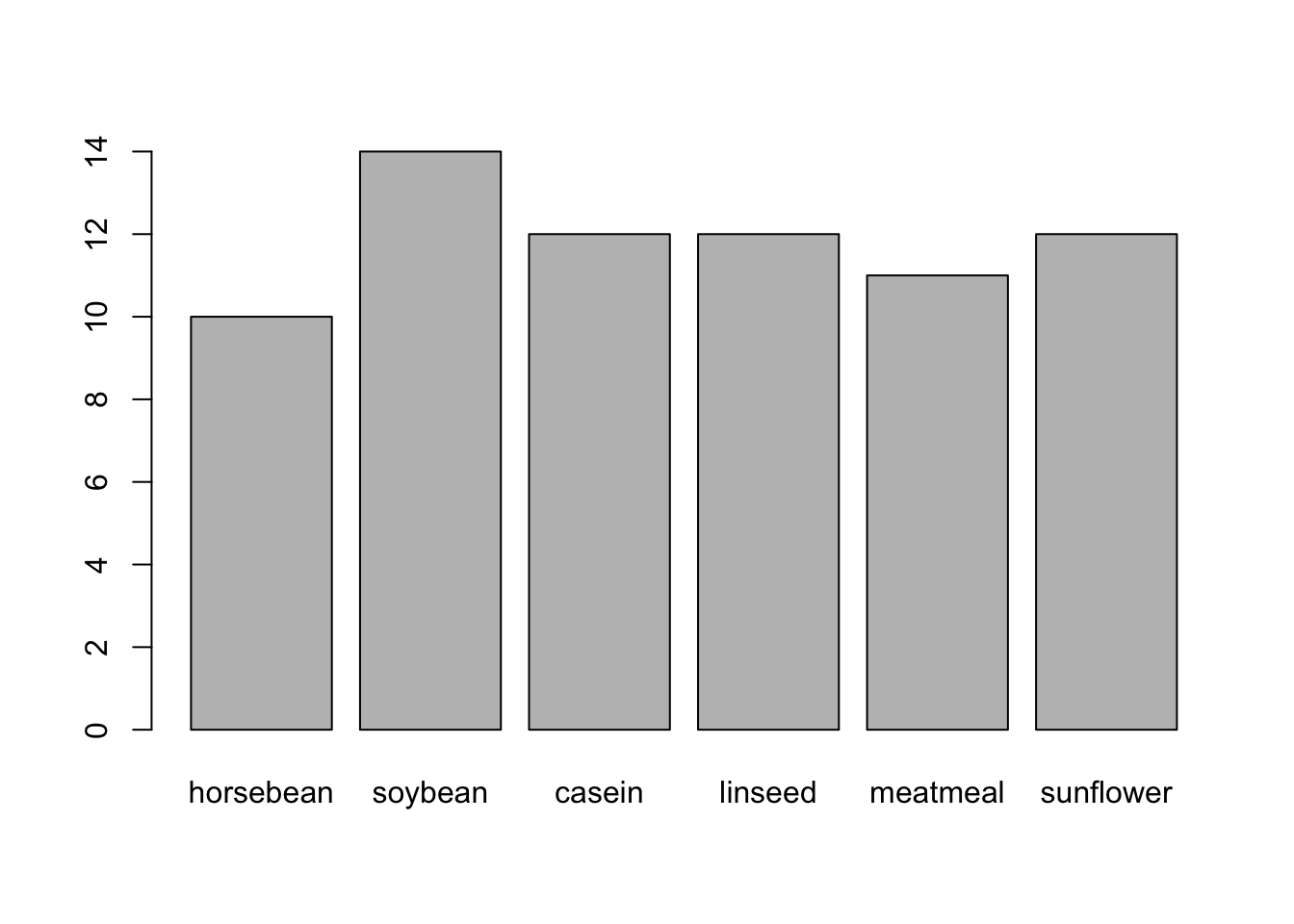

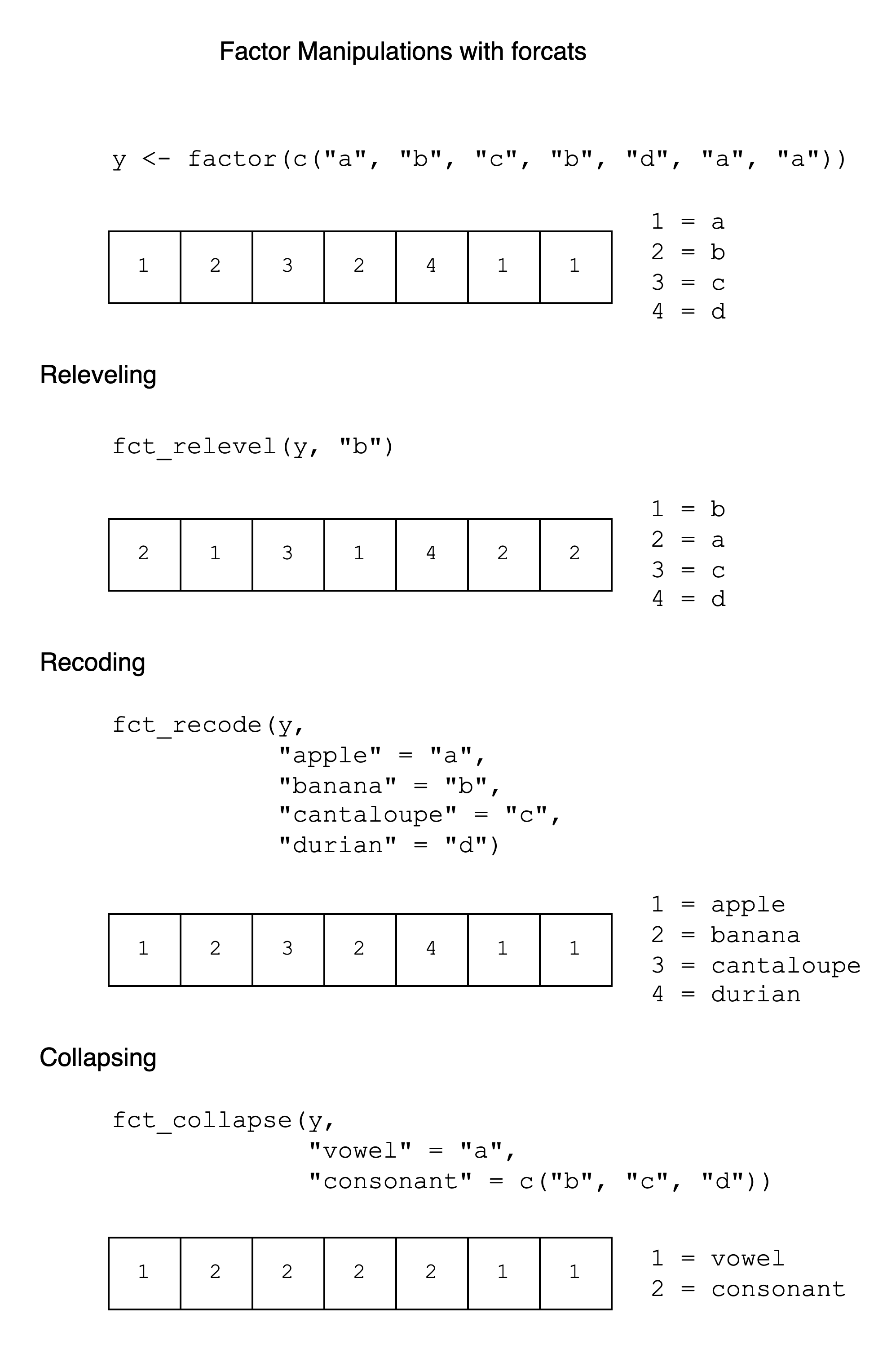
9.7 Cheat Sheet

A cheat sheet for factor manipulation is given below. It has examples of fct_relevel(), fct_recode(), and fct_collapse() with the y vector, showing the integer vector and integer-label mapping after each operation.

9.8 Exercises

9.8.1 Fundamental

Creating factors: R has a built-in list of colors accessible with colors(). Create a vector with the first letter of each color (see str_sub()). Convert it to a factor and then plot() it. Which letter is most common?

chickwts is a dataset with the weights of chickens (weight) who at different feeds (feed). Use it for exercises 2-4.

Did you make a mistake with a built-in dataset?

If we are working with external data files and make a mistake like overwriting the data, all we need to do is re-import the data.

With built-in datasets, our process looks a little different. Built-in datasets exist in the datasets or other packages. When we reference one of those objects, like penguins or chickwts, R will first look in our environment and then in the other packages we have loaded.

That means, if we have something else called penguins or chickwts in our environment, R will find that one instead of the copy in the datasets package:

chickwts <- 1
str(chickwts)

 num 1

The solution is simple. Just remove the copy in the environment with rm(), so that R will find the copy in the datasets package:

rm(chickwts)
str(chickwts)

'data.frame':   71 obs. of  2 variables:
 $ weight: num  179 160 136 227 217 168 108 124 143 140 ...
 $ feed  : Factor w/ 6 levels "casein","horsebean",..: 2 2 2 2 2 2 2 2 2 2 ...

If you make a mistake with chickwts in the exercises below, just run rm(chickwts)!

Releveling: Using the chickwts dataset, create a new column called feed_relevel from feed with code like this:
```
chickwts$feed_relevel <- fct_relevel(chickwts$feed, ...)
```
Order the levels so that running plot(chickwts$feed_relevel) returns this exact plot:
Recoding: Using the chickwts dataset, create a new column called feed_recode from feed so that plot(chickwts$feed_recode) returns this exact plot: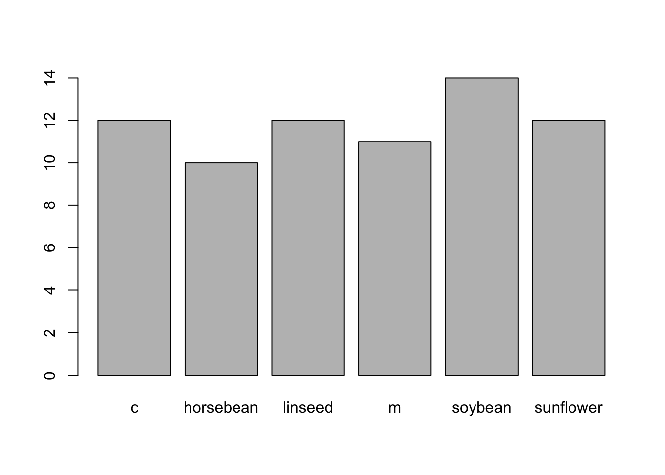
Collapsing: Using the chickwts dataset, create a new column called feed_collapse from feed so that plot(chickwts$feed_collapse) returns this exact plot: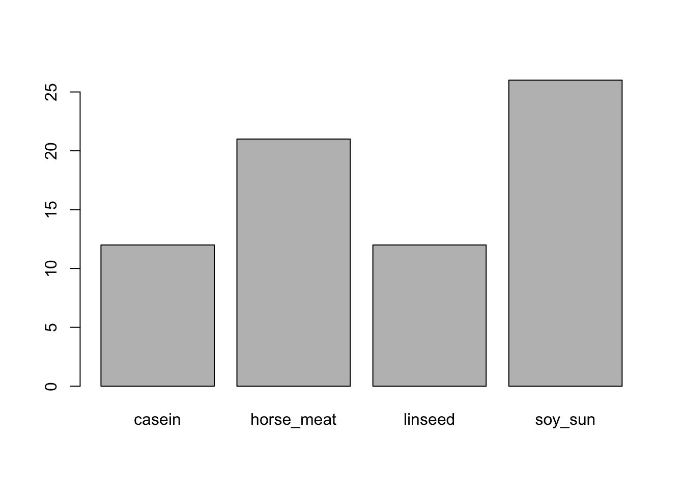

9.8.2 Extended

Relabeling with a function: Create a vector of 100 random numbers 1 to 10. Convert it to a factor. Then, rename them to start with “id” and end with “x”, like “id1x”, “id2x”, etc.
Numeric to factor: In the mtcars data, all the variables are numeric. Convert vs to a factor, where 0 has the label “V-shaped” and 1 has the label “Straight”.