1 + 3

2 + c(1, 3, 5)

c(2, 5) + c(1, 3)

c(2, 5) + c(1, 3, 5)5 Numeric Vectors
5.1 Warm-Up
What would be the result of adding together these pairs of vectors?
Make predictions before running the code.
5.2 Outcomes
Objective: To create, perform mathematical operations with, and reference elements of numeric vectors.
Why it matters: Numeric vectors are used in everyday R tasks, such as creating or manipulating variables in a dataset, plotting predicted values from a statistical model, or writing loops that repeat lines of code.
Learning outcomes:
| Fundamental Skills |
|
Key functions and operators:
c()
rep()
seq()
:
sample()
runif()
rnorm()
[ ]
5.3 Creating Vectors
Many of the vectors we use will come to us as variables in a dataframe that we import into R. At other times, we will need to create our own vectors.
5.3.1 Combine
The most basic way to create a vector is to combine elements with c(). Give the function one or more comma-separated elements:
a <- c(6, 0, 8)
a
[1] 6 0 8If we give c() vectors of varying lengths, it will “flatten” them into a one-dimensional vector, rather than returning a nested or multi-layered object:
c(a, c(2, 6, 2, 9, 9, 1, 7)) [1] 6 0 8 2 6 2 9 9 1 75.3.2 Sequence
Create a sequence of numbers with seq(). This function takes three arguments:
from: the starting valueto: the ending valueby: the step size between values
Count from 1 to 5 by 1s:
seq(1, 5, 1)[1] 1 2 3 4 5Count from 0 to 100 by 25s:
seq(0, 100, 25)[1] 0 25 50 75 100Create a vector that counts by 4 to get years with presidential elections:
seq(2000, 2028, 4)[1] 2000 2004 2008 2012 2016 2020 2024 2028If from is larger than to, make by negative to count backward:
seq(5, 1, -1)[1] 5 4 3 2 1A shortcut for counting by 1 or -1 is to use the colon operator : with the pattern from:to:
1:5[1] 1 2 3 4 55:1[1] 5 4 3 2 15.3.3 Repetition
Repeat a vector with one or more elements with the rep() function:
rep(0, times = 3)[1] 0 0 0Repeat a vector with two elements:
rep(0:1, times = 3)[1] 0 1 0 1 0 1The entire vector is repeated each time.
Change the second argument to use each instead of times so that each element is repeated before the next:
rep(0:1, each = 3)[1] 0 0 0 1 1 15.3.4 Random Numbers
R includes a number of distributions we can sample from. See ?Distributions for a list.
Take a sample of 1000 from the uniform distribution, which has a constant probability across the range [0,1]:
b <- runif(1000)Make a histogram of the data:
hist(b)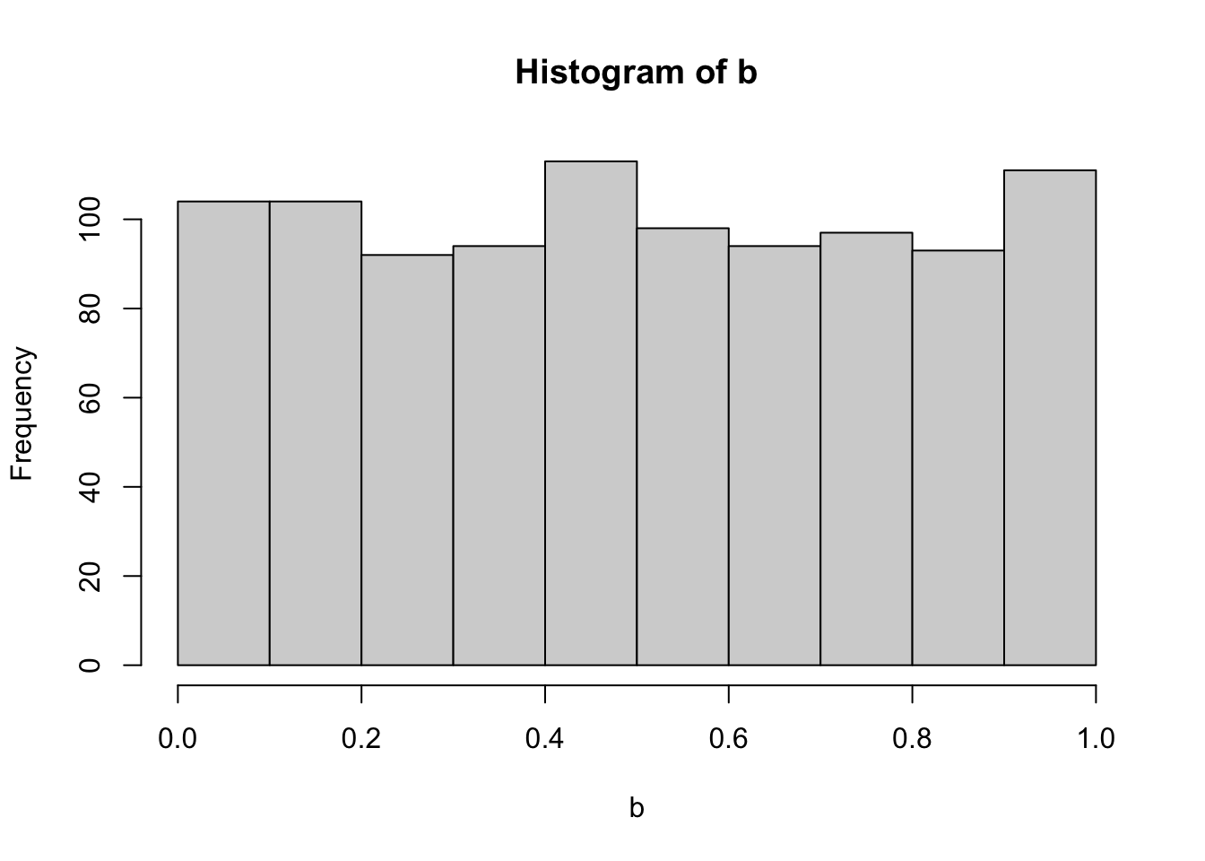
Take a sample of 1 million observations from a normal distribution. R supports scientific notation, so 1,000,000 can be written as 1e6, which means \(1 * 10^6\). (This way of writing large numbers makes updating code easier and saves us from problems where we miscount the number of 0s.)
d <- rnorm(1e6)Make a histogram:
hist(d)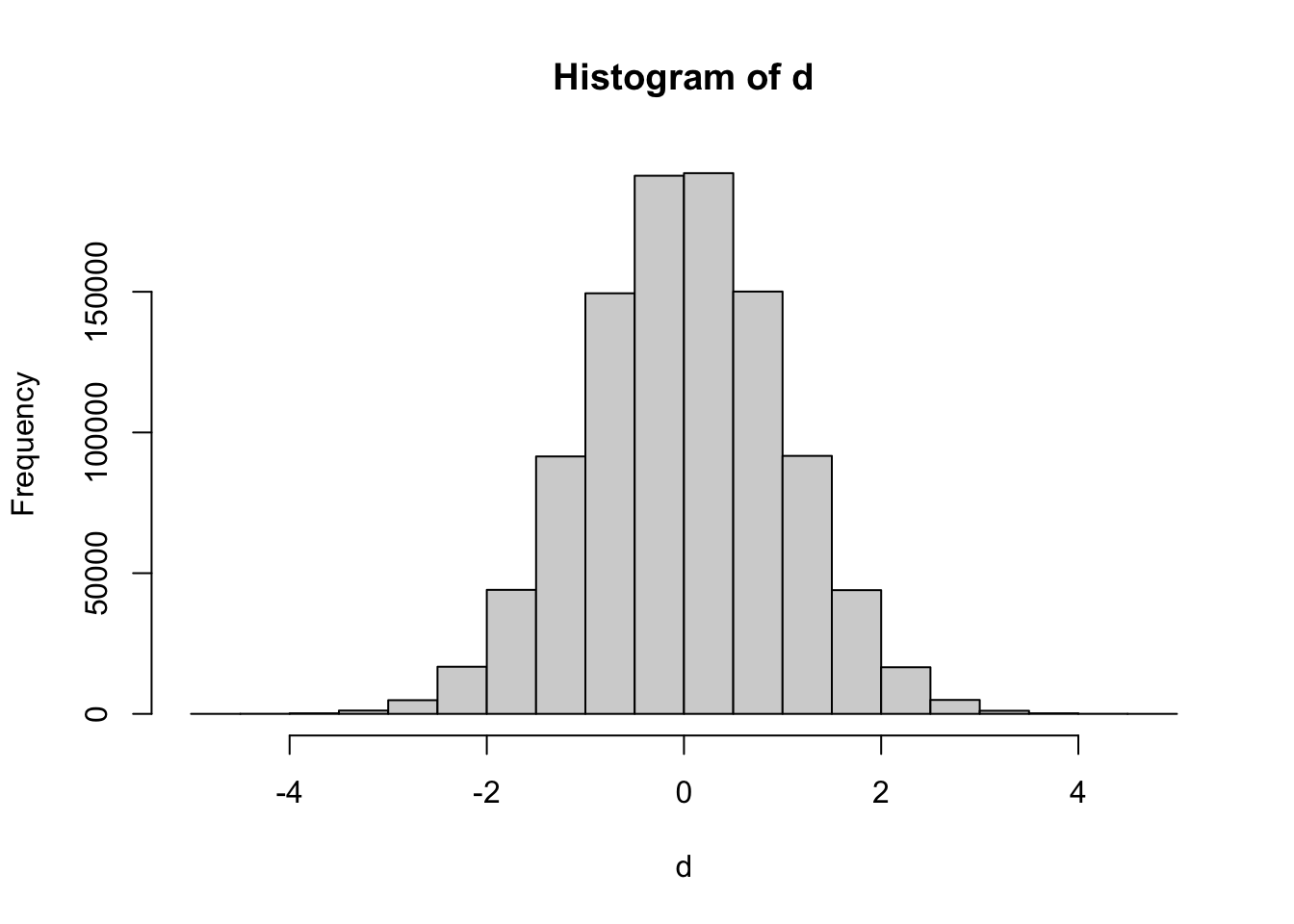
We can also sample from a known set of numbers with the sample() function. We will use three of its arguments:
x: the vector to sample fromsize: how many elements we want to samplereplace: whether we want to sample with replacement, off by default (FALSE)
Get two random numbers between 1 and 5 without replacement:
sample(1:5, 2)[1] 4 3Get 10 random numbers between 1 and 5:
sample(1:5, 10)Error in sample.int(length(x), size, replace, prob): cannot take a sample larger than the population when 'replace = FALSE'This is probably the most helpful error message you will ever see in R. It even tells you the argument you need to modify. We cannot take a sample of 10 from a population of 5 without replacing the sampled elements each time. Rerun the code with replace = TRUE:
sample(1:5, 10, replace = TRUE) [1] 4 5 2 2 5 5 5 4 1 5sample() allows us to perform simulations, such as rolling dice, which is picking two numbers between 1 and 6 with replacement:
sample(1:6, 2, replace = TRUE)[1] 3 6Our next step could be to plot the probability distribution of the sum of our two dice (is 7 most common?), or to calculate the empirical probability of rolling two of the same number (is it 1/6?). For that, we will need to write a function and a loop, something you will be ready to learn after you complete this book.
5.4 Vector Operations
We can use R’s mathematical operators to do math with vectors. First, create two vectors with the numbers 0-4 and 4-0:
e <- 0:4
f <- 4:0
Add them together:
e + f[1] 4 4 4 4 4e is c(0, 1, 2, 3, 4) and f is c(4, 3, 2, 1, 0). These vectors were “lined up” and operated on. The first element of the output is the result of adding together the first element of e and the first element of f, the second element in the output will be calculated from the second elements of e and f, and so on. e + f is essentially c(0+4, 1+3, 2+2, 3+1, 4+0), or c(4, 4, 4, 4, 4).
This element-by-element way of working with vectors is called element-wise operation.
If we have vectors of differing lengths, the shorter vector is recycled to match the length of the longer vector. Add 2 to e:
2 + e[1] 2 3 4 5 6The 2 was recycled, or reused, for each element of e. We can imagine that R first repeated the 2 so that it was as long as e (5 elements), and then it added them together:
  2 + e
= 2 + c(0, 1, 2, 3, 4)
= c(2, 2, 2, 2, 2) + c(0, 1, 2, 3, 4)
= c(2+0, 2+1, 2+2, 2+3, 2+4)
= c(2, 3, 4, 5, 6)
If the longer vector’s length is not a multiple of the shorter vector’s length, we have uneven recycling. R will perform this operation with a warning. This is undesirable because it can lead to unexpected results. The functions we will learn later when working with dataframes will instead return an error.
0:1 + eWarning in 0:1 + e: longer object length is not a multiple of shorter object
length[1] 0 2 2 4 4
Warnings Versus Errors
R returns warnings and errors when there is a possibly unexpected result from our code, or when R just thinks we should be aware of something.
The difference between the two is important. With warnings, our code still runs. If we created or modified a data object or saved a file to our computer, that will still happen with a warning. With an error, our code stops running without completing its action.
To see the difference, run the three lines below.
n <- "a"
o <- as.numeric(n)
p <- as.logic(o)
Coercing n into a numeric gives a warning because the letter “a” turned into NA, but we still get the object o because this was just a warning. Running the misspelled function as.logic() (it should be as.logical()) returns an error, and the object p is not created.
Most mathematical operators return multiple elements, one for each element in our input vectors. Some functions return a single summary statistic, like the sum, mean, or standard deviation:
sum(e)[1] 10mean(e)[1] 2sd(e)[1] 1.5811395.5 Indexing Vectors
Create another vector with sample(). If the sample size is equal to the population size and we sample without replacement, the effect is that we randomly sort the elements:
s <- sample(1:10, 10)We saw in the previous chapter how we can use numbers in square brackets to index a vector. Get the first element in s:
s[1][1] 5Now, we can use our other vector-creation skills to reference multiple elements.
Get the second, fourth, and sixth elements:
s[c(2, 4, 6)][1] 8 10 7Get those same numbers, but using seq():
s[seq(2, 6, 2)][1] 8 10 7Get the fifth element three times:
s[rep(5, times = 3)][1] 6 6 65.6 Exercises
5.6.1 Fundamental
Reproduce the following vector with
rep():[1] 1 1 1 1 1Reproduce the following vector with
seq():[1] 0 2 4 6 8 10Reproduce the following vector in at least two ways:
[1] 1 3 5 1 3 5Revisit the warm-up exercises and explain what, if anything, is being recycled in each case.
1 + 3
2 + c(1, 3, 5)
c(2, 5) + c(1, 3)
c(2, 5) + c(1, 3, 5)
Make a vector with the numbers 1 to 10. What is its type? What is its mean? Replace the first five elements with your name. What is its type now? What is its mean now?