dat <- read.csv("dataset.csv")Warning in file(file, "rt"): cannot open file 'dataset.csv': No such file or
directoryError in file(file, "rt"): cannot open the connectionWhat kinds of datasets have you used in R or other statistical software?
mtcars in R or auto in StataObjective: To import text data into R.
Why it matters: The first step in most research projects is importing a dataset into R. Data files vary in the data they include and how it is organized, so it is necessary for you to have strategies to import data in various formats.
Learning outcomes:
| Fundamental Skills | Extended Skills |
|
|
Key functions:
read.csv()
write.csv()
saveRDS()
readRDS()
getwd()
setwd()
list.files()The examples on this page require example files, which you can find at the link below.
Some browsers may try to open some file types within the browser. If that happens, right-click and select “save/download linked file as…”
If you need to work on multiple projects simultaneously, use R Projects (capital “P”). This page does not cover R Projects, but they are discussed in R for Data Science and What They Forgot to Teach You About R. In this chapter, we will assume you are only working on one project at a time, and this makes the overhead of R Projects unnecessary.
Working directories are often a foreign concept for individuals who are new to programming or whose introduction to computers has been through graphical desktops, where you point and click to open files and use dialogs to save files.
Imagine I just opened RStudio and started a script called myScript.R. I then downloaded a file (dataset.csv), which I now want to import into R. I see the file in my Downloads folder, so I tell R to import it:
dat <- read.csv("dataset.csv")Warning in file(file, "rt"): cannot open file 'dataset.csv': No such file or
directoryError in file(file, "rt"): cannot open the connectionUh-oh. I can see the file, but R cannot. Where is R looking? What does it see?
R looked for dataset.csv in its working directory.
A working directory is the folder where the software looks for files. It is the default for reading/loading and writing/saving files.
We can ask for the working directory with getwd():
getwd()[1] "/Users/bbadger/Documents/"(We can change our working directory in a few ways, and even set the default on launch in Global Options, but we will learn a better way below.)
In that directory (which we more commonly call a “folder”), what does R see? R can tell us with list.files():
list.files()[1] "myScript.R" "HW1.pdf" Notably, dataset.csv is missing from this list, and this is why R gave us the No such file or directory error when we tried to import it. How can we tell R how to find the file?
Rstudio has a wonderful functionality that, if we launch RStudio by double-clicking on a script, it will make the folder containing that script our working directory.
We need to do two things to take advantage of this functionality:
Organize files outside of R. See the sections that follow.
Launch R with scripts. First, be sure RStudio is closed. Then, launch RStudio by double-clicking on a script. Your working directory will be set to the location of that script! There is no need to set our working directory manually with setwd(). We only need to give R directions on where to read or write files relative to the location of the script, called a relative path.
A path is directions for the software on how to find a file or folder. Paths can be relative or absolute. Relative paths start from the working directory, and absolute paths start from the root directory. Here are examples of absolute paths across different operating systems:
Relative paths are preferred for most situations because they are shorter, portable, and resistant to breaking if upstream folders are renamed.
The sections that follow give suggested ways to organize your projects on your computer, ranging from very simple projects with only a couple files (such as homework assignments), to much more complex projects with many input and output files (such as dissertation research).
When to use this structure: For minor projects or homework assignments where you have only one or two of each kind of file (script, data, output, etc.).
How it is structured: All files are in a single folder.
If we have two files, myScript.R and dataset.csv, and place them in a single folder, myProject, we can visualize the structure like this:
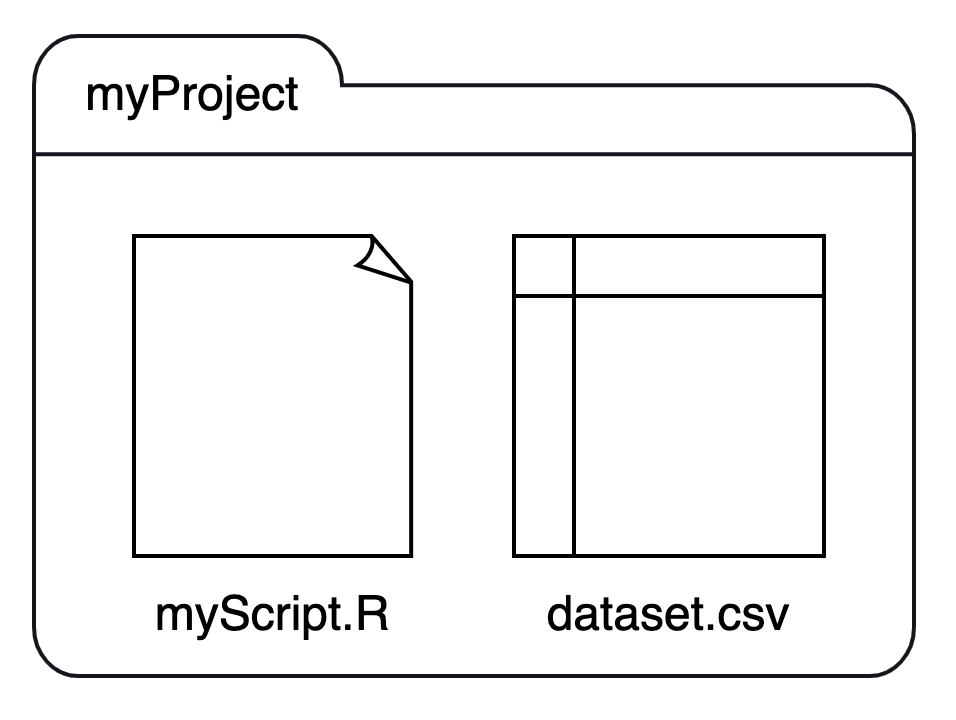
We can recast this structure as a small family tree, where myProject is a parent with two children:

Using this structure: If we launched RStudio by double-clicking on myScript.R, our working directory would be set to myProject. If we want to import dataset.csv, we can run read.csv("dataset.csv") without specifying a path before the file name.
Key idea: If we tell R to read (or write) a file without giving a path name, R will assume it is in the same folder, that it is a sibling of our script.
When to use this structure: For any substantive research, including semester projects, thesis or dissertation research, and collaborative work.
How it is structured: Files are separated into folders by their kinds, with scripts in one folder, data in a different folder, and so on. The top-level folder contains a series of folders, and those folders contain files.
Imagine we have a project of medium complexity, where we need to clean, summarize, and model multiple datasets, and produce plots with the results. This project would have started with a single script and a single data file (just like the simple structure above), but after some time, we may have created a new script for each task, downloaded more raw data files, and saved images of plots. Sooner rather than later, we should impose order on our folder structure.
We could separate the files by their types or kinds like this:
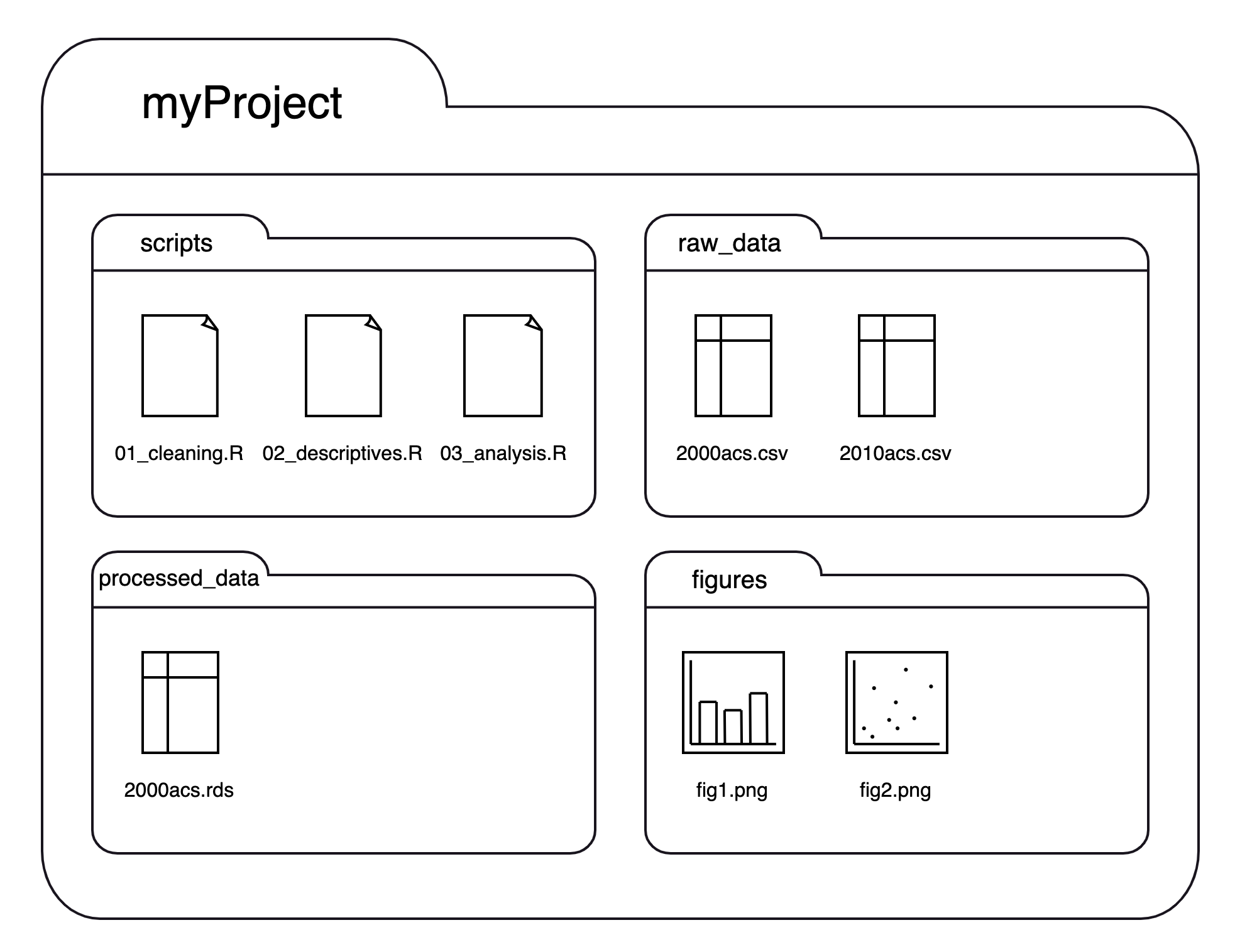
If we think of this structure as a family tree, we now have three generations, where myProject is the grandparent folder who has four children folders, each of which has 1-3 children files of their own:
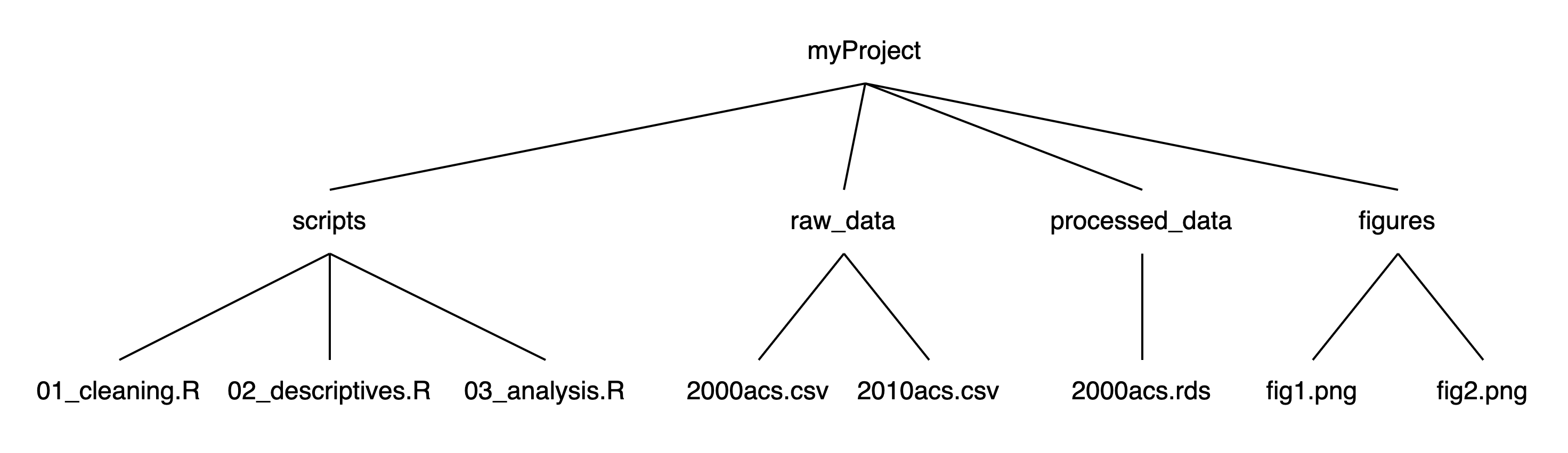
Using this structure: If we launched RStudio by double-clicking on one of the scripts in the scripts folder, our working directory would be myProject/scripts. To read a script in raw_data, we first need to tell R to (1) get out of our current folder and then (2) go into the raw_data folder. We can move out of folders with .. and into folders with their names. Each step of the path is separated by a slash (/). If we want to import 2000acs.csv, we would run read.csv("../raw_data/2000acs.csv").
Key idea: If we want R to read (or write) a file that is not a sibling of our script, we need to give it a trace of the family relation: .. to move up the family tree, and folder names to move down the tree.
We are not limited to a two-level structure for folders. We can always have more folders within folders, such as if we wanted to create subfolders within the figures folder for descriptives, margins, and diagnostics. The principles from the previous section remain the same: give slash-separated steps of how to find a file: .. to move up and folder names to move down.
To move up two folders, the path would be ../.., and to move down two folders, the path would be folder1/folder2.
If we are in myProject/scripts1/scripts2, and we want to read a CSV in myProject/data1/data2/data3, we would first need to move up two levels into myProject (the first level at which the two paths share a common ancestor), and then down three levels into data3.
To import a file called dataset.csv inside that data3 folder, we would run read.csv("../../data1/data2/data3/dataset.csv")
A typical project begins by importing a dataset from your computer into R as a dataframe. A typical file type might be a plain text file (such as a CSV), an Excel workbook, or a data file exported by another statistical software (such as a Stata .dta file).
The examples below import a series of data files that you can find by clicking this link. To run the code below, place the files into a directory called “data” that is in the working directory. To follow along, be sure that the “data” file is in your working directory. To check what R “sees”, run list.files() and verify that the data folder is there. If it is not, see the section Setting the Working Directory above.
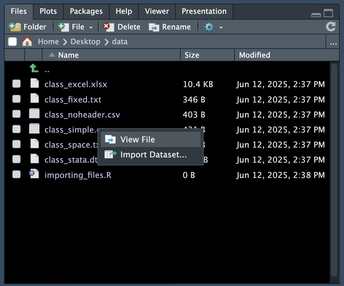
Text files come in many forms. The first thing you should do is to read any documentation that accompanies the file. Then, use RStudio to browse the file. In the Files pane, navigate to the data folder and then click on the name of a file. Some files will open with a single click, and for others you may need to click “View File”:
When you look at the file, look for a few things:
Metadata and extra text
Observation delimiter
Data value delimiter
Missing values
NA, ., -99, or BBBBBBB. There may be more than one missing value indicator that represent different types of missingness (e.g., -8 and -9), or different missing data codes in different columns.Open the file class_simple.csv in the viewer. The first few lines look like this:
Name,Sex,Age,Height,Weight
Alfred,M,14,69,112.5
Alice,F,13,56.5,84
Barbara,F,13,65.3,98
Carol,F,14,62.8,102.5
Henry,M,14,63.5,102.5
In this file,
Data like this is very easy to read into R with the read.csv() function:
class_simple <- read.csv("data/class_simple.csv")
head(class_simple)
Name Sex Age Height Weight
1 Alfred M 14 69.0 112.5
2 Alice F 13 56.5 84.0
3 Barbara F 13 65.3 98.0
4 Carol F 14 62.8 102.5
5 Henry M 14 63.5 102.5
6 James M 12 57.3 83.0str(class_simple)'data.frame': 19 obs. of 5 variables:
$ Name : chr "Alfred" "Alice" "Barbara" "Carol" ...
$ Sex : chr "M" "F" "F" "F" ...
$ Age : int 14 13 13 14 14 12 12 15 13 12 ...
$ Height: num 69 56.5 65.3 62.8 63.5 57.3 59.8 62.5 62.5 59 ...
$ Weight: num 112 84 98 102 102 ...For space-delimited data, we can use a related function, read.table(). The underlying function is the same as read.csv() but with different argument defaults. The defaults of read.table() are to assume spaces delimiting values and no header in the data.
The first few lines of class_space.txt look like this:
Name Sex Age Height Weight
Alfred M 14 69 112.5
Alice F 13 56.5 84
Barbara F 13 65.3 98
Carol F 14 62.8 102.5
Henry M 14 63.5 102.5
Here we have a header with variable names, which we need to indicate.
class_space <- read.table("data/class_space.txt", header = T)
str(class_space)
'data.frame': 19 obs. of 5 variables:
$ Name : chr "Alfred" "Alice" "Barbara" "Carol" ...
$ Sex : chr "M" "F" "F" "F" ...
$ Age : int 14 13 13 14 14 12 12 15 13 12 ...
$ Height: num 69 56.5 65.3 62.8 63.5 57.3 59.8 62.5 62.5 59 ...
$ Weight: num 112 84 98 102 102 ...Alternatively, we could use read.csv(), which assumes a comma separator (incorrect) and a header (correct). Change the delimiter argument but leave the header argument as-is:
class_space <- read.csv("data/class_space.txt", sep = " ")
str(class_space)
'data.frame': 19 obs. of 5 variables:
$ Name : chr "Alfred" "Alice" "Barbara" "Carol" ...
$ Sex : chr "M" "F" "F" "F" ...
$ Age : int 14 13 13 14 14 12 12 15 13 12 ...
$ Height: num 69 56.5 65.3 62.8 63.5 57.3 59.8 62.5 62.5 59 ...
$ Weight: num 112 84 98 102 102 ...The choice between read.csv() and read.table() is arbitrary. You may choose to always use one over the other and change argument defaults as needed. Or, you can choose to use whichever one’s defaults are closer to the dataset at hand.
Now open the file class_noheader.csv. The first few lines look like this:
Alfred,M,14,69,112.5
Alice,F,13,56.5,84
Barbara,F,13,65.3,98
Carol,F,14,62.8,102.5
Henry,M,14,63.5,102.5
James,M,12,57.3,83
The default use of read.csv() assumes the first line is variable names, resulting in some nonsense names:
class_noheader <- read.csv("data/class_noheader.csv")
str(class_noheader)
'data.frame': 18 obs. of 5 variables:
$ Alfred: chr "Alice" "Barbara" "Carol" "Henry" ...
$ M : chr "F" "F" "F" "M" ...
$ X14 : int 13 13 14 14 12 12 15 13 12 11 ...
$ X69 : num 56.5 65.3 62.8 63.5 57.3 59.8 62.5 62.5 59 51.3 ...
$ X112.5: num 84 98 102 102 83 ...To tell R that the first row is data and not variable names, specify header = F:
class_noheader <- read.csv("data/class_noheader.csv", header = F)
str(class_noheader)
'data.frame': 19 obs. of 5 variables:
$ V1: chr "Alfred" "Alice" "Barbara" "Carol" ...
$ V2: chr "M" "F" "F" "F" ...
$ V3: int 14 13 13 14 14 12 12 15 13 12 ...
$ V4: num 69 56.5 65.3 62.8 63.5 57.3 59.8 62.5 62.5 59 ...
$ V5: num 112 84 98 102 102 ...This results in variables named V1, V2, etc. We can name them upon importing with the col.names argument, or rename them later with the rename() function, which we will learn in the next chapter.
class_noheader <-
  read.csv("data/class_noheader.csv",
           header = F,
           col.names = c("Name", "Sex", "Age",
                         "Height", "Weight"))

str(class_noheader)
'data.frame': 19 obs. of 5 variables:
$ Name : chr "Alfred" "Alice" "Barbara" "Carol" ...
$ Sex : chr "M" "F" "F" "F" ...
$ Age : int 14 13 13 14 14 12 12 15 13 12 ...
$ Height: num 69 56.5 65.3 62.8 63.5 57.3 59.8 62.5 62.5 59 ...
$ Weight: num 112 84 98 102 102 ...Next, open the file class_missing.csv. The first few lines look like this:
"Name","Sex","Age","Height","Weight"
"Alfred","M",14,69,112.5
"Alice","F",-99,56.5,84
"Barbara",-99,-99,65.3,98
"Carol","F",14,62.8,-99
"Henry","M",14,63.5,102.5
Here we have a missing value code of -99 for Age in the second observation, and more missing values in other rows.
If missing values are coded as blanks (delimiters with nothing in between) or NA, R will automatically interpret them as missing. If we have another missing value, we need to specify that in the na.strings argument when importing the dataset:
class_missing <-
  read.csv("data/class_missing.csv",
           na.strings = "-99")

head(class_missing)
Name Sex Age Height Weight
1 Alfred M 14 69.0 112.5
2 Alice F NA 56.5 84.0
3 Barbara <NA> NA 65.3 98.0
4 Carol F 14 62.8 NA
5 Henry M 14 63.5 102.5
6 James M 12 57.3 83.0Data in fixed columns can be difficult to identify from merely looking at the file. Files in fixed-width format require documentation that specifies the file structure, column names, and column widths.
The first few lines of class_fixed.txt look like this:
Alfred M1469  112.5
Alice  F1356.584
BarbaraF1365.398
Carol  F1462.8102.5
Henry  M1463.5102.5
James  M1257.383
Here we need to know how many columns each variable occupies, including spaces. The documentation file for this data file may look something like this:
Var    Positions Length Type
Name   1-7       7      String
Sex    8         1      String
Age    9-10      2      Numeric
Height 11-14     4      Numeric
Weight 15-19     5      Numeric
The read.fwf() function is used for importing fixed-width text. It has a widths argument that takes a numeric vector with the number of characters for each variable. Here, we can use the values in the Length column of the documentation for the widths argument, and the names in the Var column for the col.names argument:
class_fixed <-
  read.fwf("data/class_fixed.txt",
           widths = c(7, 1, 2, 4, 5),
           col.names = c("Name", "Sex", "Age",
                         "Height", "Weight"))

head(class_fixed)
Name Sex Age Height Weight
1 Alfred M 14 69.0 112.5
2 Alice F 13 56.5 84.0
3 Barbara F 13 65.3 98.0
4 Carol F 14 62.8 102.5
5 Henry M 14 63.5 102.5
6 James M 12 57.3 83.0Excel workbooks are another common format for data files.
Any data wrangling we do in Excel, like renaming columns or calculating new ones, is neither recorded nor easily reproducible without re-clicking through menu options.
Rather than cleaning your data in Excel, you should import your data into R as early as possible so that you have a paper trail of all the work you do with your data.
Load the readxl library, which was installed with the tidyverse but not loaded with library(tidyverse):
library(readxl)The read folder has the one-sheet workbook, class_excel.xlsx. Import it with the read_excel() function:
class_excel <- read_excel("data/class_excel.xlsx")New names:
• `` -> `...2`
• `` -> `...3`
• `` -> `...4`
• `` -> `...5`
• `` -> `...6`
• `` -> `...7`
• `` -> `...8`
• `` -> `...9`
• `` -> `...10`
• `` -> `...11`
• `` -> `...12`
• `` -> `...13`
• `` -> `...14`head(class_excel)# A tibble: 6 × 14
This dataset contains …¹ ...2 ...3 ...4 ...5 ...6 ...7 ...8 ...9 ...10
<chr> <chr> <chr> <chr> <chr> <lgl> <chr> <chr> <dbl> <dbl>
1 <NA> <NA> <NA> <NA> <NA> NA <NA> Age NA NA
2 <NA> <NA> <NA> <NA> <NA> NA <NA> 11 12 13
3 Name Sex Age Heig… Weig… NA Aver… 54.4 59.4 61.4
4 Alfred M 14 69 112.5 NA <NA> <NA> NA NA
5 Alice F 13 56.5 84 NA <NA> <NA> NA NA
6 Barbara F 13 65.3 98 NA <NA> <NA> NA NA
# ℹ abbreviated name:
# ¹`This dataset contains characteristics of a class of 19 students.`
# ℹ 4 more variables: ...11 <dbl>, ...12 <dbl>, ...13 <dbl>, ...14 <chr>Uh-oh.
This Excel file has explanatory text at the top and a pivot table to the right of the dataset. Excel workbooks are often more complicated than your average CSV since they can contain multiple sheets, and a single sheet will often have extra metadata above, below, or next to the main dataset, and some sheets even have multiple datasets on a single sheet! The readxl library has functions for all of these situations and will allow you to do things like import specific sheets and cell ranges. Read more in the readxl documentation.
For class_excel.xlsx, we need to skip content at the top and to the right. If we just had text at the top to skip, we could use the skip argument of read_excel(). Here, we need to use the range argument to specify which cell range includes our data, which is A4:E23:
class_excel <-
  read_excel("data/class_excel.xlsx",
             range = "A4:E23")

head(class_excel)
# A tibble: 6 × 5
Name Sex Age Height Weight
<chr> <chr> <dbl> <dbl> <dbl>
1 Alfred M 14 69 112.
2 Alice F 13 56.5 84
3 Barbara F 13 65.3 98
4 Carol F 14 62.8 102.
5 Henry M 14 63.5 102.
6 James M 12 57.3 83 Sometimes you may need to use data from SAS, SPSS, or Stata into R. You may run into this if your colleagues use these programs while you use R, or if you are downloading a public dataset and they only offer downloads in one or more of these formats.
To import the binary data files used by these programs, load the haven library, which was also installed with the tidyverse but not loaded with library(tidyverse):
library(haven)The read folder has the file class_stata.dta, and the .dta extension tells us it is a Stata file. Use the read_dta() function to import it:
class_stata <- read_dta("data/class_stata.dta")
str(class_stata)
tibble [19 × 5] (S3: tbl_df/tbl/data.frame)
$ Name : chr [1:19] "Alfred" "Alice" "Barbara" "Carol" ...
..- attr(*, "format.stata")= chr "%-9s"
$ Sex : chr [1:19] "M" "F" "F" "F" ...
..- attr(*, "format.stata")= chr "%-9s"
$ Age : num [1:19] 14 13 13 14 14 12 12 15 13 12 ...
..- attr(*, "format.stata")= chr "%10.0g"
$ Height: num [1:19] 69 56.5 65.3 62.8 63.5 57.3 59.8 62.5 62.5 59 ...
..- attr(*, "format.stata")= chr "%10.0g"
$ Weight: num [1:19] 112 84 98 102 102 ...
..- attr(*, "format.stata")= chr "%10.0g"Files from other programs may contain data that R dataframes typically do not have, such as value and variable labels. The haven package has functions for working with these types of metadata. Read more in the haven documentation.
After you have read in and manipulated your data in R, you should save your data. As you might have guessed, the opposite of read.csv() is write.csv().
The write.csv() function has the default option of row.names = T, which will create a column with our row names. Since we did not name the rows in class_simple, they contain the default vector of 1:nrow(class_simple) by default. Turn this option off with row.names = F.
write.csv(class_simple, "class_simple.csv", row.names = F)To customize the separators and file format, see ?write.csv.
You may also choose to save your data in the RDS format. This file type has several advantages:
The primary disadvantage of RDS files is that you cannot easily preview the file in application such as Excel or a text editor.
saveRDS(class_simple, file = "class_simple.rds")To load the file back into R,
dat <- readRDS("class_simple.rds")Run this code to save two files to your working directory. Then, read them back into R. Hint: Do not trust the extension to tell you how the file is structured. View the file contents to determine its delimiter, presence of header, etc.
write.table(ChickWeight, "chick1.txt", sep = ",", row.names = F)
write.table(ChickWeight, "chick2.txt", row.names = F)
Save airquality as a CSV file.
Save chickwts as an RDS file.
Print your working directory to the console.
Create a folder called “import_practice” on your computer and move the files you saved in exercises 2 and 3 into this folder. Place this folder either in your working directory or as a sibling folder to your working directory. Without changing your working directory, specify relative paths to read them into R.
Run this code, which creates a CSV in your working directory called “class_scores.csv”, where a value of -99 means missing. Read it back into R and ensure that the missing data is coded as NA.
data.frame(id = sample(1:10, 100, replace = T),
           score = sample(c(90:100, -99), 100, replace = T)) |>
  write.csv("class_scores.csv", row.names = F)
A fixed-width version of mtcars is available at https://sscc.wisc.edu/sscc/pubs/dwr/data/import_extended.txt. Read it into R, following the information in the codebook at https://sscc.wisc.edu/sscc/pubs/dwr/data/import_extended_codebook.txt. Compare it to mtcars to ensure it matches.